【1頁】
Experiment for Positive Externalities
——Is Coase Theorem applicable to the Positive Externalities?——
Naoyuki Kaneda
1. Introduction
There are many arguments in economic and legal research about Coase theorem. In 1960, Coase took an example of negative externalities and argued that the efficiency is achieved regardless of the liability rule. He took the example of straying cattle which destroy crops growing on neighboring land. In his example, a farmer and a cattle-raiser are operating on neighboring properties. He further supposes that, without any fencing between the properties, an increase in the size of the cattle-raiser's herd increases the total damage of the farmer's crop. He concluded that the ultimate result is independent of the legal position (whether the cattle-raiser is liable or not for damage), if the pricing system is assumed to work without costs.
The experimental literature supports Coase's argument. Hoffman and Spitzer (1982) conducted experiments with bargaining and side payments. Their experimental design simulates the negative externalities in pollution problem. We are aware of few experiments in positive externalities in this literature. This paper deals with bargaining with positive externalities. The experiments in this paper try to simulate the R&D activities among several companies. The results of R&D activities of one firm can easily be replicated by others at lower costs. In this paper's experimental design, each firm may spend its resources on R&D activities, but the results of successful R&D activities benefit all firms, regardless of whether a particular firm spends its resources on that activity. This is an example of positive externalities. My major interests are whether players in the experiments bargain for their benefits and achieve the joint payoff maximum. I deal with two kinds of experiments under positive externalities: 1) Coasian Bargaining with certainty, 2) Coasian bargaining with uncertainty.
2. Literature Review
Hoffman and Spitzer (1982) report that their research, in which they used bargaining and side payments for verification, supports the Coase theorem. Coase concluded that a change in liability rule would leave the agents' production and consumption decisions unchanged and economically efficient in the following framework:
(a) two agents to each externality (and bargain), (b) perfect knowledge of one another's (convex) 【2頁】production and profit or utility functions, (c) competitive markets, (d) zero transaction costs, (e) costless court system, (f) profit-maximizing producers and expected utility-maximizing consumers, (g) no wealth effects, (h) agents will strike mutually advantageous bargains in the absence of transaction costs.
(Hoffman and Spitzer, 1982: 73)
Hoffman and Spitzer verified that subjects achieved their joint payoff maximum under 1) full information, 2) existence of controller and 3) two and three-party bargaining.
Harrison and Mckee (1985) criticized the conclusion of Hoffman and Spitzer (1982). They insist that Coase theorem suggests that subjects achieve both 1) joint payoff maximum and 2) mutually advantageous bargaining (i.e., controller receives more than or equal to individual maximum). They also insist that Hoffman and Spitzer (1982) only verified the achievement of joint payoff maximum in the experiment and that the controllers in fact failed to exploit their bargaining positions in some situations. Harrison and Mckee suggest that those results might be interpreted as altruistic behavior. They conducted the experiment with increased social surplus (i.e., the difference between the maximum payoff and the next best alternative), finding that the equal splits are reduced in their experiments.
Hoffman and Spitzer (1985) reasoned that the controller failed to exploit their advantage because they did not correctly perceive it. They found that controllers make more profits with the first instruction with the expression “earns the right to be (controller)” than with the second instruction with the expression “is designated to be controller.”
Harrison and Mckee (1985) also changed the nature of property rights and proved that there is indeed an externality problem. They observed that joint payoff maximum is not pervasive in their setting and concluded that the existence of controller and side payments is crucial to achieve joint payoff maximum.
Shogren (1992) examined Coasian bargaining under uncertain payoff streams. Subjects bargained over both ex ante lottery and the ex post reward. Shogren used the traditional “controller” scheme, which is different from the positive externality scheme in this paper, and showed that 87% of all agreements were Pareto-efficient. However, only 7.3% were mutually advantageous and 85 percent of all agreements split the reward equally.
Isaac and Reynolds (1988) demonstrated that the R&D activities (i.e., the mean number of draws in their setting) are larger without positive externalities (with “full appropriabilities”) than with positive externalities (with “partial appropriabilities”). Their scheme, however, does not include the negotiations and side payments.
3. Experimental Design
In Coase theorem literature, most papers deal with negative externalities and few papers deal with the positive externalities. This paper will attempt to reveal the behaviors specific to positive externalities in Coasian bargaining.
A major difference in Coasian bargaining under negative externalities and under positive externalities is the existence of the “controller.” In Hoffman and Spitzer (1982), the experimenter flips a coin to 【3頁】decide which individual will be the “controller.” Either player may become a “polluter” in the context of negative externalities of a pollution problem. But in positive externalities of “R&D activities,” there are no controllers.
Either player has an option to spend their resources on R&D activities, but neither player can force others to spend their resources on R&D activities. With respect to this issue, the experiments for positive externalities are quite different from the experiments of negative externalities.
In this paper, I deal with two-player experiments. Each subject has the option to spend money on R&D activities. In this sense, each subject is a “controller” for his/her own decision. If one subject spends her money on R&D activities without uncertainty, all the subjects will get the benefits of the R&D activities because the benefits of the results of one firm can easily be imitated by others. If both subjects spend money on R&D activities under certain payoffs, neither party gets the benefits for positive externalities.
We conducted the three-party experiment under certainty. The major motivation of the experiment under this condition is to verify the outcome, if the number of subjects is increased. As Hoffman and Spitzer (1982) mentioned, “many observers have theoretically assumed that imperfect information or multiple agents in a bargain will tend to preclude contracting by the affected parties.” Thus, we have to test the results under increased number of subjects.
We also conducted the experiment under uncertain payoffs, whereas Shogren (1992) studied bargaining for negative externalities under uncertainty, we focused on positive externalities under uncertainty. Another difference between Shogren (1992) and ours is the informational setting: in Shogren, subjects have only limited information: in our experiment, subjects have full information.
Under uncertain payoffs, binomial lotteries are introduced for R&D activities. In our experiments, if R&D activities are successful, all subjects benefit from R&D activities.
Next, we will discuss some conditions that we will need to induce the appropriate bargaining under uncertainty.
In the following discussion, “Spending-Spending” indicates a situation in which both players spend their resources on R&D activities, while “Spending-No spending” indicates a situation in which player A spends her resources but player B does not. “No spending-Spending” indicates a situation in which player B spends her resources but player A does not. “No spending-No spending” indicates that neither player spends their resources on R&D activities.
One condition to inducing negotiations among subjects is that subjects are better off spending their resources on R&D activities. Otherwise, they are better off without spending their resources in R&D activities and they do not have externalities.
Another issue for the parameter setting is that expected payoff for “Spending-Spending” should be less than the expected payoff for both “Spending-No spending” and “No spending-Spending.” Otherwise, subjects do not have incentives to negotiate for better payoffs. They simply achieve better payoffs in “Spending-Spending” without negotiations.
Thus, to induce negotiation for R&D activities, we need the following conditions for symmetrical probabilities:
【4頁】
1. In the “Not spending- Not spending” situation, each player is worse off than he or she would have been spending some points for R&D activities while other player is not spending. Otherwise, the best strategy for each player is not to spend points on R&D activities.
2. The expected payoff for “Spending-Spending” for two subjects is smaller than the aggregate expected points both for “Spending-No spending” and “No spending-Spending.”
Suppose that each player's payoff for “No spending ? No spending” is (0,0). And denote the payment for “R&D activities,” additional payoff for the successful “R&D activities” and the probability for success as a, b and p, respectively.
Then, the above conditions can be expressed as:
1. a<2bp
2. a>2bp(1-p)
For example, b=5, a=3 and p=0.4 satisfies the above conditions. But in this parameter setting, we have to be careful about risk averse behavior of subjects. If the expected payoff for the “Not spending” strategy is close to the expected payoff for “Spending- Spending” or “Not spending- Spending,” subjects might choose the riskless “Not spending” strategy.
In the experiment above, I introduced the asymmetrical probability for R&D activities. With this setting, I can avoid the incentive problems in the above example. Specifically, the probability of success for player A is 80% and the probability of success for player B is 10%.
4. Instructions
a. Certainty setting
First, I will verify that the Pareto-optimal outcomes are achieved and that the mutually advantageous situation is achieved in this setting. Agreement forms similar to Hoffman and Spitzer (1982) are used in the following experiments.
Instruction for Two Person Experiments
Following the general explanation similar to Hoffman and Spitzer (1982), subjects are shown the following instruction. The experimenter read the instruction orally after a few minutes.
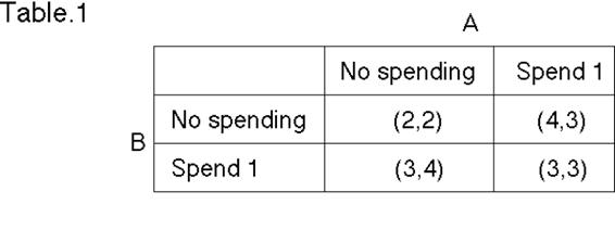
You will be asked to make one choice. The cash value to you of the outcome in the table below is given. (See Table 1 in Appendix 1.) You have two points at the beginning of the experiment. You have an option to spend 1 for to get 2 points. But if you spend 1 for your self, the other player also gets 2 points. The other player has the same option to spend 1 and get 2 points. In the example shown below, you might be person B. If you spend 1 and person A does not spend 1, you will get additional 1 and person A gets additional 2. Your payoff sheets list not only the value of each number to you, but also the value of each number to other participant. Each of you will make your own decision. After both of you make decisions and inform the monitor, who will stop the experiment and pay both participants. You and other 【5頁】participant may attempt to influence each other to reach mutually beneficial decisions. You and other participant may offer to pay part or all of his of her earnings to each other.
Are there any questions? We ask you to answer the questions on the attached sheet to make sure you understand the instructions.
Question
1. Suppose you are player A. If you spend 1, how many points does each player get?
2. Suppose you are player A. If only player B spends 1, how many points do you get?
3. If both players spend 1, how many points does each player get?
The experiment is conducted in sequential setting. Six pairs of subjects make two decisions each, in sequence. The subjects know that they would make two decisions together. All bargaining is face to face. The object is to simulate coordination on R&D activities between two firms in the same industry.
Instruction for Three Person Experiments
As the subjects arrive at a designated room they are randomly assigned the letters A, B, or C. Each triad was placed in a separate room, with monitor being the only other person present. The monitor provides the following set of instructions to the subjects, who first read the instructions silently and then listen to the monitor, read them aloud.
Following the general explanation similar to Hoffman and Spitzer (1982), subjects are shown the following instruction.
You will be asked to make one choice. The cash value of the ending points is given to you. You have two points at the beginning of the experiment. You have an option to spend 1 for to get 2 points. But if you spend 1 for your self, the other two players also get 2 points. If anyone of one or two or three persons spends 1, every person gets 2 points. If no one spends a point, no one gets anything. You know not only your payoff but also other player's payoff for each outcome.
Are there any questions? We ask you to answer the questions on the attached sheet to make sure you understand the instructions.
Question
1. Suppose you are player A. If you spend 1, how many additional points do the other players get?
2. Suppose you are player A. If player B spends 1, how many additional points you and player C get?
3. Suppose you are player A. If both player B and player C spend 1, how many points do you get?
4. If all three players spend 1, how many points does each player get?
【6頁】
Objective of the experiment is to simulate coordination on R&D activities among three firms in the same industry.
b. Uncertainty setting
Instruction for Two Person Experiments
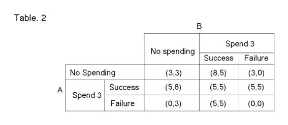
You will be asked to make one choice. You have 3 points at the beginning of the experiment. You have an option to spend 3 to draw a lottery. But be careful. The probability of success in lotteries varies for player A and for player B. If player A spends 3 to draw a lottery and gets 1 on random number table, both players get 5 points. Player B has the similar option to spend 3 and draw a lottery. If player B spends 3 to draw a lottery, and if player B gets 1 through 8, both players get 5. If both players spend 3 and either or both of players get successful numbers, both players get 5.
For example, suppose that you are person B. If you spend 3 and person A does not spend 3, and if you get 1 through 8 in random number table, you get additional 2 after paying 3 and person A gets additional 5. If you spend 3 and person A does not spend 3, and if you get 9 or 10 on random number table, you lose 3 with the initial payment and other person A gets nothing. If both of you draw lotteries paying 3, and either of you or both of you get successful numbers in the random number table, both of you get additional 2 points after paying 3. If both of you draw lotteries paying 3, and neither of you gets successful numbers in the random number table, both of you get nothing and end up with nothing. Your payoff sheets list not only the value of each outcome to you, but also the value of each outcome to other participant. (See Table 2 in Appendix 1.) Each of you will make your own decision. After both of you make decisions and inform the monitor, person(s) who paid 3 will draw lotteries and the monitor will stop experiment and pay both participants. You and other participant may attempt to influence each other to reach mutually beneficial decisions. You and other participant may offer to pay part or all of his of her earnings to each other.
Are there any questions? We ask you to answer the questions on the attached sheet to make sure you understand the instructions.
Questions
1. Suppose you are player A. If you do not spend 3 to draw and player B spends 3 to draw a lottery, what is the expected point for you?
2. Suppose you are player A. If both you and player B spend 3 to draw lotteries, what is the expected point for you?
3. Suppose you are player A. If you spend 3 to draw a lottery and player B does not spend 3 to draw a lottery, what is the expected point for you?
4. If both of you do not spend 3, what is your expected point?
The objective of the experiment is to simulate the coordination on R&D activities under different probabilities of success between two firms.
【7頁】
5. Hypothesis
I have the following hypotheses for these experiments.
H1: Under the positive externalities scheme, the parties will choose the joint payoff maximum, even in the absence of unilateral property rights.
If H1 holds given that subjects are allowed to make transfer of monetary value, the experiments support the Coase theorem in the positive externalities situation. In the positive externalities setting, the “controller” is embedded in the scheme and we do not need to designate the “controller” in the experiment. Harrison and Mckee concluded that the establishment of unilateral property rights (i.e., the existence of controller in the experiment) increases the number of joint payoff maximums. I will test this hypothesis to verify behaviors under positive externalities because we do not have controllers in this setting.
H2: Under certain payoffs with positive externalities, subjects split their payoffs equally.
Hoffman and Spitzer (1982) showed that the “controller” gets the individual maximum or more in some situations. These experiments would test whether the person who spends money is better off by the bargaining. In the positive externalities setting, there is no controller in the experiment, and no subject is supposed to get the individual payoff maximum.
H3: Even under uncertain payoffs with positive externalities, the parties will choose the joint payoff maximum.
H4: Under uncertain payoffs with positive externalities, players split the reward equally in their agreement.
Shogren (1991) showed that nearly 87% of all agreements were Pareto efficient. However, only 7.3% were mutually advantageous and nearly 85% of all agreements split the reward equally. I will test the similar hypothesis under positive externalities.
6. Experimental Results
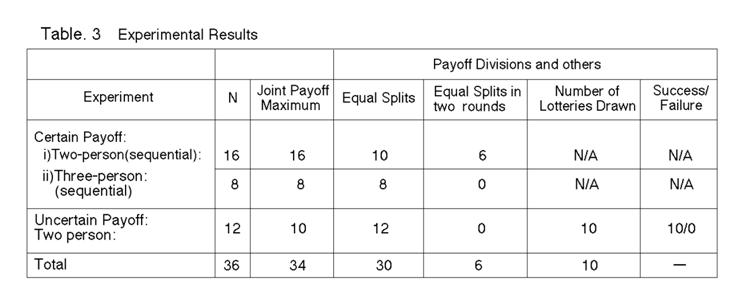
In the results of two-person experiment, sixteen out of sixteen experiments achieve joint payoff maximum, which seems to support Hypothesis 1. See Table 3 in Appendix 1 for the detailed results of the experiment.
Table 3 also shows the payoff divisions. Ten out of sixteen pairs split the payoff equally. Six out of sixteen pairs split their payoff in two rounds. In other words, they simply keep their payoff for each 【8頁】round, but each subject's aggregate payoff is the same for one sequence. Given that the equal splits in two rounds are the same as the equal splits, all the experiments show the “equal splits” of their payoffs. It represents a significant difference between this experiment and those of negative externalities. In the negative externalities settings, they almost always have controllers with the bargaining power to enforce their choices. Harrison and Mckee (1985) showed that controllers tend to get a larger payoff for the large payoffs. Subjects in the positive externalities settings lack this kind of enforcement: each player has the same bargaining power in the experiments, and it is quite natural that subjects split their payoff equally. Because there is no controller in this paper's setting, nobody achieves the individual payoff maximum.
The second line in Table 3 shows the results for three-party experiments, which also show that all pairs achieve the joint payoff maximum. These results are similar to those of Hoffman and Spitzer (1982), but the results of payoff divisions are quite different. Eight out of eight results show equal splits in these experiments, while in Hoffman and Spitzer (1982), three out of twenty-one made equal splits for full-information in a single controller case and nine out of sixteen made equal splits for full-information in a joint controller setting. Once again, the difference is made by the existence of controller(s). In the positive externalities setting, no one has bargaining power to enforce the individually better payoff.
In the positive externalities setting, the existence of a controller is not crucial to achieving the joint payoff maximum. Is the unilateral property right (i.e., the existence of controller) really necessary to achieve joint payoff maximum in the Coasian bargaining under negative externalities?
To answer this question, we review the results of the experiments in Harrison and Mckee (1985). To test the hypothesis (H6) that the establishment of unilateral property rights increases the number of joint payoff maximum, Harrison and Mckee compared the results under two different conditions: no property rights (NPR) and unilateral property rights (UPR). Under the NPR condition, side payments are prohibited and there is no controller. Under the UPR condition, sidepayments are allowed and there is a controller.
Harrison and Mckee concluded that H6 was strongly supported by the experiment when they compared the results under UPR and results under NPR. But it is a confusing argument. They have another condition called joint property rights (JPR) in their experiment. Under JPR, there is no controller but two players jointly choose the number and divide the total payoffs.
Harrison and Mckee should compare the results under UPR and JPR conditions to test the hypothesis (H6), because both conditions allow the transfer of the property but differ in the existence of controllers. In fact, they admit that there is no significant difference between the efficiency properties (i.e., the number of joint payoff maximum) of JPR and UPR conditions. They should conclude that there is not significant effect to the efficiency (i.e., the number of joint payoff maximum) with respect to the existence of controller.
On the other hand, results under NPR and JPR conditions provide the significant difference: they imply the importance of “transferable property rights” rather than the existence of a “controller.”
Considering this analysis, we suggest that the existence of controller is not crucial in the Coasian bargaining.
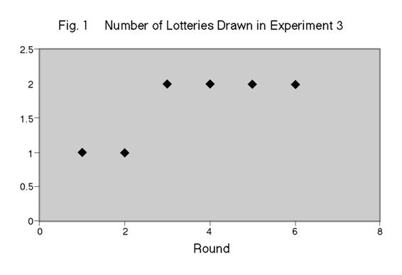
Next, we will discuss our results under uncertainty. The third line in Table 3 shows the results of uncertain payoffs. Ten out of twelve pairs achieve the expected joint payoff maximum. To induce negotia【9頁】tions, each player has a different probability for successful R&D activities. Even in the asymmetrical probabilities of success, each subject seems to have a same bargaining power in these experiments. Compared to the results of Shogren (1991), the results of these experiments show the better efficiency in terms of Pareto-optimality. One reason for the better efficiency is that subjects have full information about the payoff and probability of successful R&D activities in these experiments. In the experiments of Shogren (1991), subjects have limited information about the probabilities of payoff of other subject. Similar to Shogren (1991), most of the results in our experiment show the equal payoffs, which might be interpreted as risk sharing rather than bargaining for payoffs.
7. Concluding remarks and extensions
The experiments of positive externalities support Coase's theoretical proposition. Under the full information setting, most of agreements are Pareto-optimal for both certain payoffs and uncertain payoffs. Subjects achieve the joint payoff maximum in our experiment. These results indicate that the unilateral property rights (i.e., the existence of controller) are not crucial to the efficiency in the bargaining under positive externalities.
The absence of controllers in the positive externalities setting gives equal bargaining power to subjects. As a result, no one has the bargaining power to achieve individual payoff maximum.
Our further analysis of the results in Harrison and Mckee (1985) implies that the unilateral property rights are not crucial even for the bargaining under negative externalities.
We may consider the following extensions of this paper.
1. What would be the results of the experiment if social surplus (i.e., the difference between the maximum payoff and the next best alternative) is increased? Do subjects still split their payoffs?
2. Under uncertain payoffs, what would happen if each player has asymmetrical payoff between under successful R&D activities and failed ones? (In our experiment, the differences of payoffs between two players are the same in the successful R&D and failed one. It facilitates the negotiation between two parties.)
3. What if side payments are not allowed in my experiment?
Reference
Baumol, W., 1972, “On Taxation and the Control of Externalities,” The American Economic Review, 62, 307
Bigelow, J. P., 1993, “Inducing Efficiency: Externalities, Missing Markets, and the Coase Theorem,” International Economic Review, 34, 335
Canterbery, E. R. and A. Marvasti, 1992, “The Coase Theorem as a Negative Externality,” Journal of 【10頁】Economic Issues, 26, 1179
Coase, R.H., 1960, “The Problem of Social Cost,” Journal of Law and Economics, 3. 1-44
Davis, O. and A. Whinston, 1962, “Externalities, Welfare and the Theory of Game,” Journal of Political Economy, 70, 241
Harrison, G. and M. Mckee, 1985, “Experimental Evaluation of the Coase Theorem,” Journal of Law and Economics, 18, 653-670
Hoffman, E. and M. Spitzer, 1982, “The Coase Theorem: Some experimental Test,” Journal of Law and Economics, 15, 73-98
Isaac, R. and S. Reynolds, 1992, “Schumpeterian Competition in Experimental Markets,” Journal of Economic Behavior and Organization, 17, 59-100
Isaac, R. and S. Reynolds, 1988, “Appropriability and Market Structure in a Stochastic Invention Model,” The Quarterly Journal of Economics, 647-671
Randall, A., 1974, “Coasian Externality Theory in a Policy Context,” Natural Resource Journal, 14, 35-54
Shogren, J., 1992, “An Experiment on Coasian bargaining over ex ante lotteries and ex post rewards,” Journal of Economic Behavior and Organization, 17, 153-169.
【11頁】
Apendix 1
【12頁】