【1頁】

Analysts’ Forecast Revisions and Errors around Executive Turnover:

Do Japanese Firms Manage Earnings around Turnovers?

Naoyuki Kaneda

1.　Introduction

Existing literature about earnings management examine the accounting variables to find the earnings management in U. S. firms. Pourciau (1993) finds some inconclusive evidence. Murphy and Zimmerman (1993) conclude that turnover-related changes in several accrual and expenditure accounts are due mostly to poor performance. Since CEO turnovers are typically preceded by poor performance (Warner et al. 1988, Weisbach, 1988), it is difficult to distinguish the earnings effect due to poor performance and management discretion. It is unlikely to be fruitful to use more elaborate accrual estimation model such as model used in Jones (1991), because Dechow et al. (1995) show that discretionary accruals estimated from such models are also correlated with firm performance.
　 In this paper, we take an indirect approach by examining the earnings expectation change around CEO turnover for Japanese firms. An advantage of this approach is that such an analysis effectively controls the confounding effects of firm performance. Analyst earnings forecasts prior to the turnover announcements should have already incorporated the poor firm performance over a relatively long period. Thus, any systematic abnormal forecast revisions during the short window around turnover announcements can be attributed to the expected discretionary behavior of the new manager.
　 An assumption in the above discussion is that analysts rationally expect any possible earnings management related to CEO turnovers and incorporate such information in their earnings forecast revisions in a timely fashion. The validity of the analyst rationality assumption is itself of interest and subject to empirical testing. Past studies have found evidence of systematic forecast errors inconsistent with rational expectations. Although various rationality-based explanations have been proposed (Francis,1997; Gu and Wu, 2002), no single factor, or factors, has been able to fully explain the systematic forecast errors.
　 An advantage of our event approach is that it is relatively easy to isolate the turnover-related effects, and any systematic patterns of forecast revisions or forecast errors around turnovers can be used to draw 【2 頁】 inferences on analysts’ forecast behavior. Based on a priori predictions of CEO turnover-related management discretionary behavior, we can differentiate analysts’ behavior under different assumptions.In particular, if the new CEOs systematically manage earnings downward, we expect rational analysts to revise their earnings forecasts in the same direction. However, if analysts are irrational in that they either cannot understand the implications of CEO turnovers, or they do not update their forecasts in a timely fashion, then both their forecast bias and forecast accuracy will deteriorate. On the other hand, if earnings management is more active after CEO turnovers but not in a particular direction, we will not observe systematic revisions or increase in forecast biases, but forecast accuracy will be worsened. Finally, if there are no earnings management related to CEO turnovers, neither analyst forecast revisions nor forecast bias/accuracy will be affected.
　 Kaneda (2002) examine analysts’ earnings forecast revisions and errors around CEO turnovers for U. S. firms. They do not find the significant downward revisions around CEO turnovers. They do find the optimistic forecast biases for the event year. Analysts might make the optimistic forecasts before turnover announcements. It might be an indication that managements manipulate earnings downward in the event year.
　 Existing literature of earnings management use accrual estimation models to examine accounting variables in Japanese firms. Shuto (2001) examines discretionary accruals using Jones model and modified Jones model. It is important to examine analysts’ forecast around CEO turnovers to eliminate the confounding effect of firm performance.
　 Kang and Shivdasani (1995) examine the role of corporate governance mechanisms during top executive turnovers in Japanese firms. They find that firm performance improves significantly after outside succession. Following Shuto (2001), we examine the data for the sub sample of firms whose top executives are replaced by outsiders.
　 The remainder of the paper is organized as follows. Section 2 describes hypothesis development. Section 3 describes the research design and data. Section 4 presents the results. Section 5 concludes the paper.

2.　Hypothesis Development

Following Kaneda (2002), we have two major issues in this research, the behavior of CEOs and the behavior of analysts. We analyze several situations considering these two major issues in the hypotheses development.
　 First, we analyze a situation where CEOs manage earnings downward after turnovers. If CEOs manage earnings downward, what do analysts observe? If analysts are rational, they expect that CEOs manage earnings downward in the transition year. Thus, analysts revise their earnings forecast accordingly in the short period to reflect their judgment. On the other hand, analysts revise their forecasts less optimistically even without such judgment toward the end of fiscal year in general. Considering the nature of forecast revisions, we expect larger negative forecast revisions right after turnover announcements.
　 When security analysts get new information about the firm, they may reflect that information immediately or on a relevant future date. We have two hypotheses as follows:

【3頁】

H1a: Forecast revisions around the announcement of CEO turnovers for earnings of the transition years are not statistically larger than those in the non-event years.
H1b: Forecast revisions around the expected date of CEO turnovers for earnings of the transition years are not statistically larger than those in the non-event years.

H1b is also tested, because analysts in Japan might reflect the turnover related information around the expected date of turnover rather than the date of turnover announcement.

If CEOs manage earnings downward and analysts are not rational, they do not revise their forecast accordingly. And if analysts do not revise their forecast with turnover announcement, their forecast errors will deteriorate accordingly. This analysis leads us to the following hypotheses.

H2: Forecast biases do not deteriorate for the event year.

H3: Forecast accuracies do not deteriorate for the event year.

“Forecast bias” is defined as the difference between the actual earnings and earnings forecast deflated by stock price one month before a turnover announcement. If the earnings forecast is optimistic, the forecast bias is negative. Forecast accuracy is the absolute value of forecast bias.
　 If CEOs do manage earnings but not in a particular direction, what kind of revisions do analysts observe? Even if analysts are rational, we should not see systematic revisions in their forecasts. If CEOs do not manage earnings in a particular direction, analysts’ forecast bias should not deteriorate. In this case, we would observe the larger forecast errors in absolute magnitude and a decline in forecast accuracy. We also test H2 and H3 about analysts forecasts around the expected turnover in addition to the date of turnover announcement.
　 Following the existing literature, we also test the hypotheses with the subset of data of voluntary and non-voluntary turnovers. Furthermore, we test the hypotheses with the subset of data of turnovers whose CEOs are replaced by outsiders/insiders. Shuto (2001) finds the significant results with sample whose CEOs are replaced by outsiders. We also examine this sub-sample.

3.　Research design

We took a sample from both around turnover announcements and around the expected turnover dates and found that we do not find the significant results for the forecast revisions around turnover announcement. Thus, we decided to focus on the results surrounding the expected turnover date in the following sections.
　 We define the “event year” as the year when the newly hired CEOs can manipulate earnings. Since listed firms publish their audited financial statements a few months after the fiscal year-end, we include turnover dates within two months after the fiscal year-end into that fiscal year ¹⁾.
　 We begin our analysis by taking the forecast frequencies around the expected turnover dates for each analyst. If analysts revise their forecasts after turnover dates, we expect to observe more forecast 【 4 頁】 revisions after that dates. We compare analysts’ forecast revisions and forecast errors in event years with those in non-event years. We considered two windows for analysts’ forecast revisions: one month and three month. We find few analysts’ revisions for one-month window. Thus, we concentrate on the analysis in three-month windows in the following sections.
　 Following Kaneda (2002), we estimate “normal revisions” using the method of Jain (1992). If analysts are rational and new CEOs indeed manage earnings downward, we should see the larger downward revisions in the event year than those in non-event year. If we regress forecast revisions on dummy variables and abnormal returns in Jain’s model, we can test the hypotheses in terms of coefficients on dummy variables. We make the cross-sectional regression in the following form:
(1)　Δ FREV=f(Dummy, ABEVT, ABPRE, ABPOST), where Δ FREV means forecast revision, ABEVT, ABPRE, and ABPOST are abnormal stock returns in a period surrounding the announcement date, abnormal stock returns in a pre-event period and a postevent period.
　 Regarding the tests for forecast bias and forecast accuracy, our tests are also based on both nonparametric tests and multi-variate analysis. We use the model of Gu and Wu (2002) for the analysis of forecast biases. We use the model of Brown (1999) for the analysis of forecast accuracy. We choose the TRAC model in Brown (1999). We also examine the forecast biases before turnover announcements.
　 Following Jain (1992), we include the abnormal return prior to the turnover and after the turnover, because the stock market tends to reflect new information prior to the event and it might take time for investors to digest the new information. We calculate the abnormal return using a market model with equally weighted market return including all distributions. In the expression (1), Δ FREV is the mean of the last forecast revision made by analysts for each firm in the event window. The event date is the top executive turnover announcement date or the expected turnover date on the Nikkei Telecom database. More details of the search process will be given at the start of the next section.
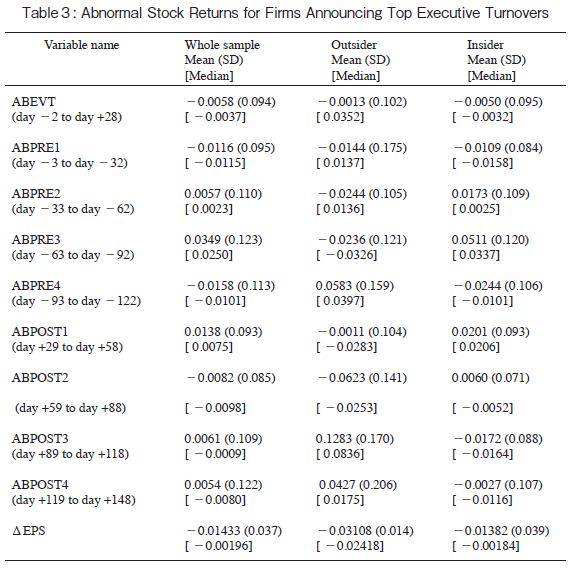
　 The abnormal return (ABEVT) is abnormal stock return derived from the market model from day-2 to day+28. The pre-event period consists of a 120-day period from day-3 to day-122. The post-event period consists of a 120-day period from day+29 to day+148. The subperiods are defined as follows:

ABPRE1: abnormal returns from day -3 to -32
ABPRE2: abnormal returns from day -33 to -62
ABPRE3: abnormal returns from day -63 to -92
ABPRE4: abnormal returns from day -93 to -122
ABPOST1: abnormal returns from day +29 to +58
ABPOST2: abnormal returns from day +59 to +88
ABPOST3: abnormal returns from day +89 to +118
ABPOST4: abnormal returns from day +119 to +148

We take forecast revisions as the difference of mean earnings forecasts before and after the announcement. We use 250 days (day -373 to day -123) to estimate the market model for the purpose of abnormal returns. We make the regressions of expression (1) for a whole sample with a turnover dummy and with voluntary and non-voluntary dummies. We also make regressions for a whole sample with a turnover dummy and with ‘outsider turnover’ dummies. We consider firms whose CEOs are replaced by 【 5 頁】outsiders as “outsider turnover” and other firms as “insider turnover.”
　 Following Shuto (2001), we consider CEOs as “outsiders” if they had taken the positions in the firms during the four-year period prior to taking the positions of CEOs. We consider other cases as “insider” CEOs.
　 To obtain forecast bias and forecast accuracy, we use the actual earnings per share (EPS) by I/B/E/S.
　 We get the stock price information from Toyokeizai Kabuka CD-ROM and stock return information from Nikkei Portfolio Master. We take the data of firms’ financial statements from Nikkei NEEDS. To avoid small deflator problems, we require that stock prices be larger than or equal to 100 YEN.

4.　Data Collections, Analyses, and Results

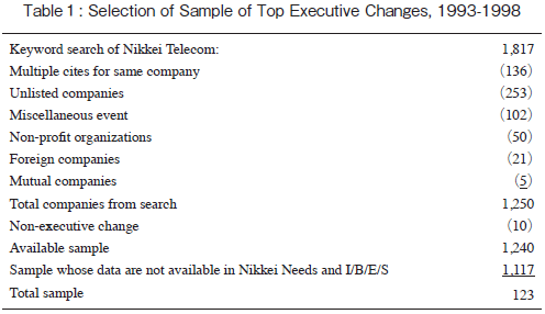
4.1.Table 1, Selection of Sample of CEO Changes: In this section, we shall elaborate on the process of data collections, analyses, and results.
　 We use the term, CEO turnover announcement, to mean the announcement of top executive turnover. We searched the top executive turnover in Nikkei Telecom database. A keyword search of the database was conducted for ‘Shacho’ (president) or Kaicho (chairman of the board) with the descriptions of ‘Kotai’ (turnover) or ‘Kainin’ (dismissal) or ‘Jinin’ (resignation) or ‘Tainin’ (retirement) or ‘Shunin’ (appointment) or ‘Shokaku’ (promotion) and so on. The search provides 1,240 companies from 1993 to 2000 as shown in Table 1. (We use the term turnover to mean “CEO turnover” and turnover announcement to mean “CEO turnover announcement.”)
　 We employ the data of Nikkei Needs and I/B/E/S database. If some data are unavailable for one turnover, it is excluded from the final sample.
　 Table 1 shows the sample selection. We get 1,817 reports in a Nikkei Telecom search. But some of them are multiple-cites and others are non-turnover events. Some are for non-profit organizations. Eliminating those irrelevant or redundant samples, the total number of firms is 1,250. We also exclude 10 events because of non-executive turnover. Price data of some samples is not available in the Toyokeizai Kabuka CD-ROM. In addition, for the analysis of analysts’ forecast revisions, we need forecast revisions both in pre-turnover windows and post-turnover windows and the final sample size is smaller. Thus, the number of CEO turnovers in the sample is 123.
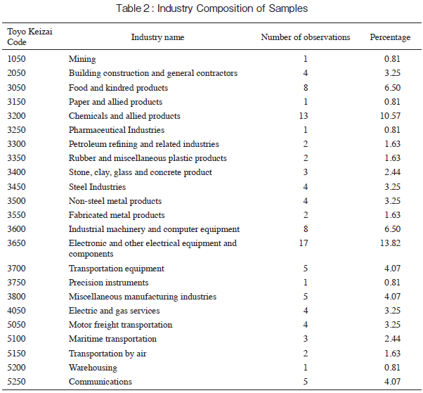
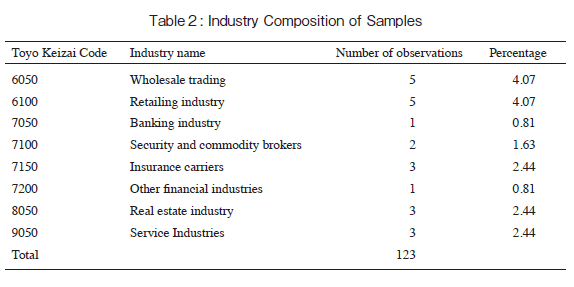
　 4.2.Table 2: Industry Composition: Here, 123 sample firms are shown in Table 2. Although we see more observations in some industries such as ‘Food and kindred products,’ ‘Chemicals and allied products,’ and ‘Electronic and other electrical equipment and components,’ the sample is fairly diversified.
　 We refer to the date in which the turnover announcement was made as the event date. The expected turnover date or, omitting “expected,” turnover date is the date mentioned in the announcement as the date the CEO is expected to take over. (Actual turnover dates were not traced since the publicly announced turnover dates are most likely be the actual turnover dates.) We use the term turnover year or transition year to mean the fiscal year that includes the expected turnover date stated in the announcement, i. e., the expected date on which the transition from the old to the new CEO takes place.
　 As mentioned in Section 3, only the results from the samples obtained using the expected turnover dates will be reported, even if those using the turnover announcement dates have been prepared but 【 6 頁】 found to have insignificant results. We also define the event year to mean, as mentioned before, the first fiscal year that includes the turnover date if extended by two months into the future. For a calendar-year company, if the turnover date is February 28, 1998, the event year is 1997 while if it is March 1, 1998, the event year is 1998. Note that all earnings and forecast data dealt with in this study are annual data.
　 4.3. Table 3, Abnormal Returns: Following Kaneda (2002), we provide a table to show the top executive turnovers as well as their announcement timing. The table shows that during the 270 days (nine 30 day periods) from 122 days before the turnover dates and 148 days after the turnover dates, firms having top executive turnovers had negative abnormal stock returns in the periods of ABPRE4, ABPRE1, ABEVT and ABPOST2. The most significant negative returns appeared in the first 30-day period (from day -122 to day -93; -0.0158). The return is significantly negative at 5% level.
　 We do not provide data for the non-voluntary and voluntary samples, since we do not find significant results for voluntary and non-voluntary samples. We do not provide the abnormal stock returns around turnover announcement, since we do not find the significant results for multivariate analysis using the method of Jain (1992) for the forecast revisions around turnover announcement.
　 Outsider turnover sample shows larger negative abnormal returns in ABPRE1, ABPRE2, ABPRE3, ABPOST1 and ABPOST2. In the second to last 30-day period, the largest positive return shows up for outsider sample (0.1283).
　 Even CEOs who had apparently resigned involuntarily tend to remain on the board in Japanese firms. Thus we conclude that Pourciau’s definition of non-voluntary turnovers is not suitable for the executive turnovers in firms in Japan. We have the following definitions for non-voluntary and voluntary turnovers. Voluntary turnovers include 1) apparent retirement which includes completion of a few terms of office, 2) top executive replaced by direct descendents, 3) CEOs older than the age of 65 years and 4) holding the title of Representative Director after turnovers, even if we do not have the description of turnover. If the article of Nikkei Telecom mentions the poor performance of the firm, we classify the turnover as non-voluntary. We exclude sample with the death of top executive from voluntary and non-voluntary sub-sample. We did not eliminate financial institutions and the regulated companies from our sample.
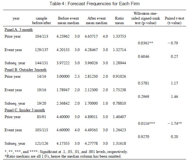
　 4.4. Table 4, Forecast Revision Frequencies: After the above overview, we now begin our analysis with the frequencies of earnings forecasts for each firm. Following Kaneda (2002), these analyses focus on the frequency of earnings forecast revisions for each firm during the pre-turnover three month period and the post-turnover three month period (Panel A).
　 These forecast data and frequencies were obtained from the I/B/E/S database for the period of 1993-2000. We collected data and grouped for each of the firms in the sample, counting the number of forecasts made by analysts during the pre- and post-turnover periods. Multiple forecasts by a given analyst in a three-month period are counted as one forecast. The ratio of the post- turnover forecast frequency over the pre-turnover forecast frequency was taken for each firm. Number of sample is larger than 123 firms for the most categories, because we need forecast revisions both in pre-turnover windows and post-turnover windows and stock price to deflate the revisions in Table5.
　 Next, the same analysis was done using the data one year earlier than the event year, taking the corresponding three month periods before and after the expected turnover date moved backward by one year. The difference between the two ratios for each firm provided a basis for 1) Wilcoxon one-sided 【 7 頁】 signed-rank test and its p-value and 2) a paired t-test and its t-values. They are listed in Table 4 as the top number in Panel A under the Wilcoxon test column and under the Paired t-test column. The same analysis was done comparing the event year and one year subsequent to the event year and p- and t-values are given as the bottom numbers in the panel under the Wilcoxon test and t-test columns.
　 Panels B shows results from the same analyses carried out for 3 month periods, not for the entire sample firms but only to those firms where CEO turnover was judged to be replaced by outsiders, where the criteria for outsiders/insiders classification was explained earlier in Section 3. Panels C shows results from the same analyses carried out for 3 month periods, not for the entire sample firms but only to those firms where CEOs are judged to be replaced by insiders.
　 One point should be pointed out. Mean ratio for “outsider 3 month” sub-sample is 1.75. On the other hand, mean ratio for prior year and subsequent years are 0.910 and 0.788 respectively. Although the difference is not statistically significant at 5%, ratio for the event year is larger than those in non-event years. We do not find the significant difference between the ratios for event-year and non-event years for the whole sample (panel A) and sub-sample for “Insider 3 month.” Kaneda (2002) find the significant difference in ratios between event-year and non-event years in the non-voluntary sub-sample. The executive turnovers seem to provoke the interests of analysts but the result is not statistically significant.
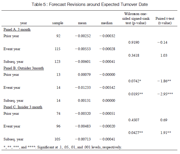
　 4.5. Table 5, Forecast Revision Amounts: Next we make analyses of forecast revisions after the expected turnover date. Descriptive statistics of forecast revisions around turnover dates are shown in Table 5. Unlike Table 4 which focuses on frequencies, Table 5 focuses on the amount of revisions around the expected turnovers. Here, we take an analysts’ per-share earnings forecast for a given firm made during the three-month window immediately after the expected turnover date and a forecast made by the same analyst for the same firm but during the three-month window immediately before the expected turnover date. If an analyst makes more than one forecast in a three-month window, the latest one is chosen. If an analyst makes forecasts only in the pre-turnover period or only in the post-turnover period, the forecast is thrown away.
　 These forecasts are then averaged for the post-turnover window for a given firm and the same is done for the pre-turnover three-month period. The post-turnover average amount less the pre-turnover average amount is then divided by the firm’s stock price at the beginning of the fiscal year. It is expressed in a fraction, indicating the level of forecast revisions.
　 The same analysis is carried out for the data one year before the turnover date. The result is then paired with the event year data and the Wilcoxon one-sided signed-rank test is applied to the pairs of data and p-value is computed as well as the paired t-test and the t-value. The same series of analysis is done comparing the event year fraction with the fraction developed for the period one year after the expected turnover date. We expect that the executive turnover is a bad news, especially if the CEOs are replaced by outsiders and that analysts will revise forecasts downward, hence a one-sided test was applied.
　 We do not find significant results for the three-month whole sample (panel A). Mean forecast revisions in the event-year shows larger negative revisions (-0.00553) compared to the mean forecast revisions in the prior year (-0.00252). On the other hand, mean forecast revisions in the subsequent year shows larger negative revisions (-0.00601) than the mean forecast revisions in the event year (-0.00553). Wilcoxon 【 8 頁】 one-sided signed-rank test and paired t-test do not indicate the significant differences. We do not find significant results for voluntary and non-voluntary subsample. Shuto (2001) does not find the significant results for non-voluntary sub-sample. It might imply that management does not manage earnings downward in non-voluntary turnovers in Japanese firms.
　 We have more interesting results for three-month outsider sub-sample. Mean forecast revisions in the event year is -0.01233. On the other hand, forecast revisions in the prior year and the subsequent year are positive and the magnitude of the revisions is much smaller (0.00079, 0.00131). Paired t-test indicates that event-year revisions have larger negative revisions at five percent level. Wilcoxon onesided signed rank tests do support this observation. Outsiders tend to replace the existing CEOs when firms have very poor performance. It might imply that management manages earnings downward for ‘outsider turnovers.
　 Panel C shows that mean forecast revisions in the event year (-0.00483) have larger negative revisions than those in the prior year (-0.00320). The non-parametric tests do not indicate that their difference is significant. The mean forecast revisions in the subsequent year for “insider” sample show larger negative revisions than those in the event year. Although we search for specific reasons, we do not find convincing explanations for these results.
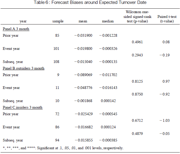
　 4.6. Table 6, Forecast Biases: Next we examine earnings forecast errors. The univariate analysis for forecast biases, defined as actual earnings less forecasted earnings, divided by the stock price at the beginning of fiscal year, is shown in Table 6.
　 We do not have particularly significant results for forecast biases presented in Table 6. For example, we have larger negative mean forecast biases in the prior year (-0.031900) than those in the event year (-0.019800) in the three-month window. If management manages earnings downward and analysts do not make sufficient downward revisions in the event year, we are supposed to have negative (i. e. optimistic) forecast biases. The results do not match with this hypothesis. We do not find the larger negative forecast biases in the event year either in the outsider sub-sample or in the insider sub-sample. We have larger forecast revisions in the outsider sub-sample but do not find the overly optimistic forecast in the same sub-sample. Kaneda (2002) find the overly optimistic forecast in the event year for nonvoluntary sub-sample. Our results show a contrast with their results in the univariate analysis.
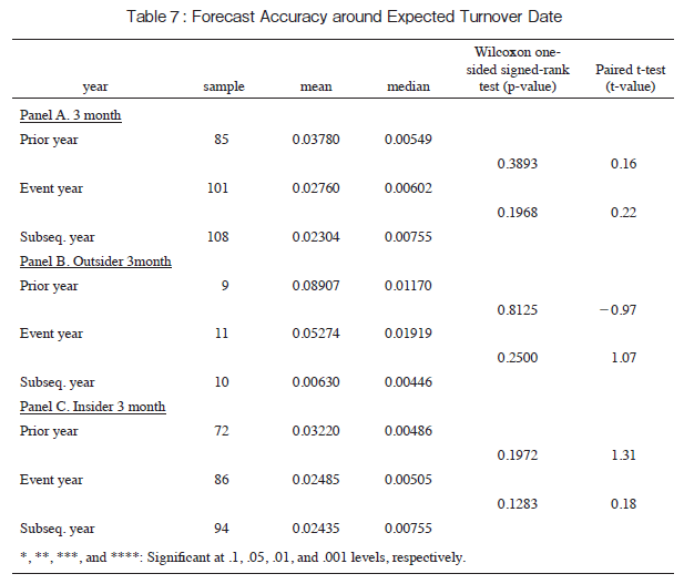
　 4.7. Table 7, Forecast Accuracies: We examine the forecast accuracy next. Table 7 shows the results of univariate analysis for forecast accuracies, defined as the absolute value of the forecast biases.
　 Mean forecast accuracy in the event year is not significantly different from those in non-event years for three-month whole sample. Non-parametric tests do not indicate the statistically significant difference. If management manages earnings downward but analysts do not reflect the information effectively, analysts’ forecast accuracy deteriorates. Panel A does not show the forecast accuracy deteriorates in the event year. Panel B shows that forecast accuracy improves in the event year compared to the forecast accuracy in the prior year. The results do not match with this story either.
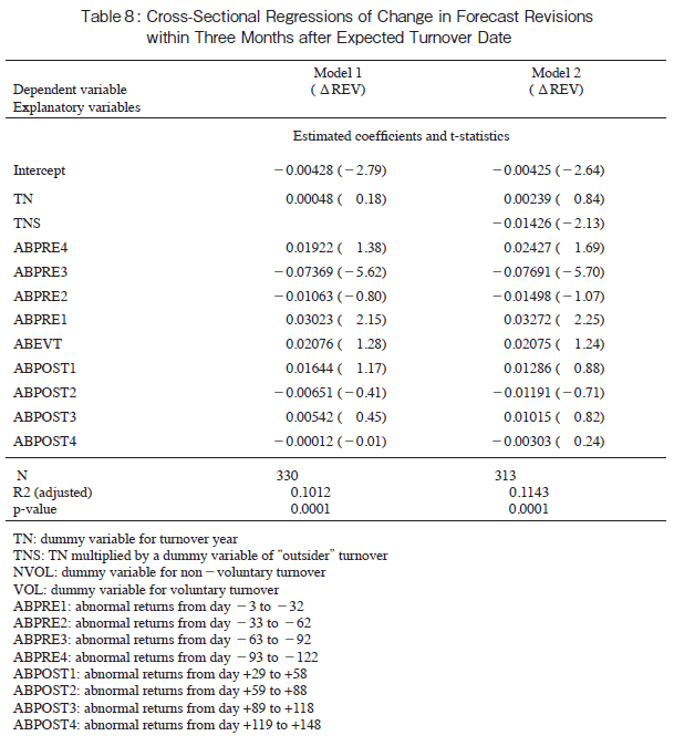
　 4.8. Table 8, Forecast Revision Regressions: As previously mentioned in Section 3, we take advantage of the method of Jain (1992) to make multi-variate analysis. In essence, we consider the “normal revision” to consider the other information reflected in the forecast revisions.
　 Table 8 shows the results for multi-variate analysis in three-month window. Model 1 uses the dummy 【 9 頁】 variable for turnover year. Model 2 uses dummy variables for turnover year and a dummy of turnover year multiplied by a dummy of “outsider” turnover (TNS). In this way, the coefficient of turnover dummy shows the effect of “insider” turnover in the event year. The coefficient of TNS dummy shows the effect of “outsider” turnover in the event year. Sum of the coefficient of turnover dummy and the coefficient of TNS dummy shows the effect of turnover year.
　 First of all, both of Model 1 and Model 2 are statistically significant. (In Model 1, p-value is 0.0001. p-value for Model 2 is 0.0001.) At least one coefficient of the independent variable is significant to explain the change in forecast revision.
　 Following Kaneda (2002), we find the significant relationship between change in earnings variable and abnormal return around the announcement. Coefficients of ABPRE3 and ABPRE1 are statistically significant. The coefficient for dummy variable is not statistically significant.
　 The second column of Table 8 shows the results for Model 2. As in Model 1, at least one independent variable is statistically significant to explain the change in forecast revisions. The coefficient of TNS dummy is statistically significant at 5% level. It implies that analysts’ forecast revisions around “outsider” turnovers shows statistically significant negative forecast revisions. If management in the firms where the top executives are replaced by outsiders manages earnings downward and analysts reflect that information in a timely manner, we observe the negative forecast revisions around turnovers. The results match with this story. Since multi-variate analysis around turnover announcements does not show the statistically significant results, it might imply that financial analysts reflect the information in their forecast when the executives take office.
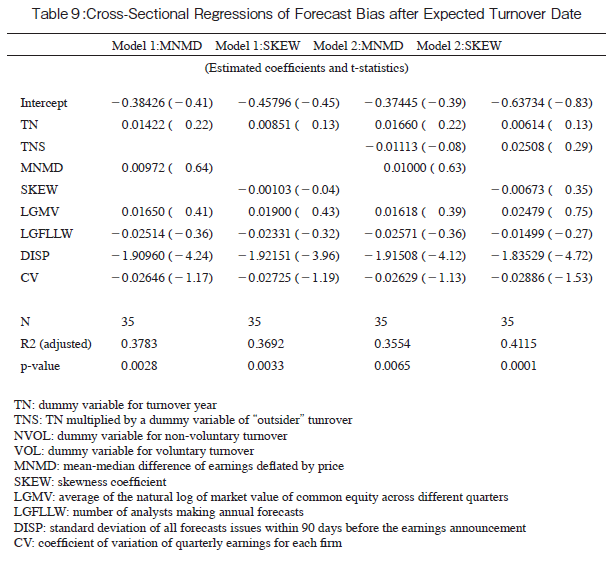
　 4.9. Table 9, Forecast Bias Regressions: Following Gu and Wu (2002), we use mean-median difference, skewness, natural logarithm of market value, and number of analysts making annual forecasts for the multi-variate analysis. Results are presented in Table 9.
　 Table 9 presents the results for three-month window. Model 1 represents the results with a dummy variable for event year. Model 2 represents the results with a dummy variable for turnover year and a dummy of turnover year multiplied by a dummy of “outsider” dummy (TNS). Gu and Wu (2002) used two different parameters for skewness (MNMD and SKEW), and we have two different regressions for each model.
　 First of all, p-value for Model 1 regressions using parameter MNMD and SKEW are statistically significant (0.0028 and 0.0033, respectively) at 1% level. The coefficients for skewness (SKEW and MNMD), LGMV and LGFLLW are not statistically significant. The coefficient of turnover dummy is not significant.
　 Results for regressions for Model 2 are right-most two columns in Table 9. First of all, two regressions for Model 2 are statistically significant at 1% level. p-values are 0.0065 and 0.0001 respectively. The coefficients of TNS dummy are not statistically significant. In the analysis of forecast revisions for the “outsider” sample, we do find the significant revisions in the event year. We do not have some negative forecast biases in the event year for “outsider” sample. Analysts might revise their forecasts of the firms where CEOs are replaced by outsiders and their forecasts are not statistically optimistic.
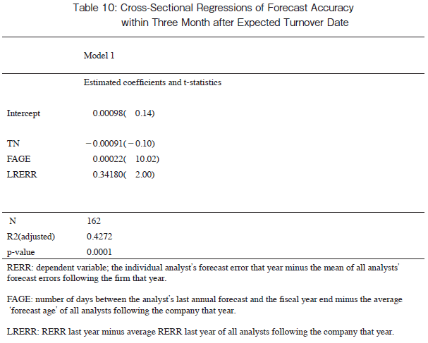
　 4.10. Table 10, Forecast Accuracy Regressions: We follow Brown (1999) for the multi-variate analysis of forecast accuracies. Following Kaneda (2002), we use two-factor TRAC model. The results 【 10 頁】 of regressions using TRAC model are presented in Table 10.
　 Data for model 2, which includes turnover dummy and TNS dummy, are not shown in Table 10, since we do not have enough data for “outsider” sample. Hence, only the results for Model 1 are shown in Table 10.
　 Regression results of Model 1 are statistically significant (p-values being 0.0001.) As in the previous multi-variate analysis, Model 1 uses dummy variable for turnover years. As shown in Table 10, the coefficient of turnover dummy is not significant at ten percent level. It implies that forecast accuracies in event years do not deteriorate significantly with respect to the forecast accuracies in non-event years.
　 The results may be more compatible with non earnings management for the whole sample, since we do not have significant ones for forecast accuracy.
　 4.11. Forecast Biases before Turnover date: We conducted the univariate analysis and multi-variate analysis of forecast biases before expected turnover dates. If management manipulate earnings downward and analysts revise their forecasts, we have even more optimistic forecasts in the period immediately before the expected turnover dates. But we do not find the significant results in these analyses. (Results are not shown in tables.)
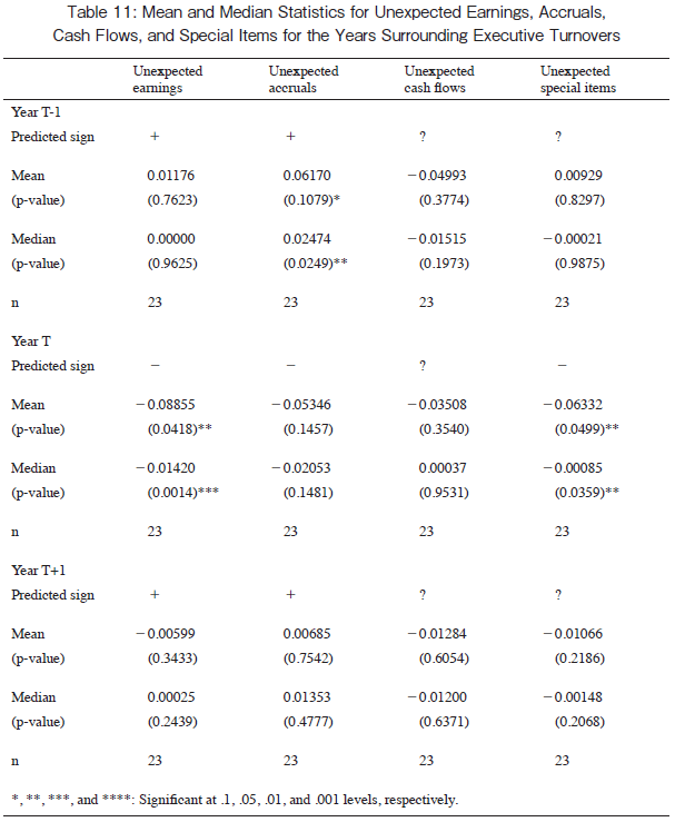
　 4.12. Table 11 Unexpected Earnings, Accruals, Cash Flows, and Special Items: We also replicate the results of Pourciau for sub sample of ’outsider’ turnover. The results are shown in Table 11. Since we do not need forecast revisions both in pre-turnover windows and post-turnover windows for this replication, the sample size in Table 11 is larger than that in Table 5 Panel B. Similar to Pourciau (1993), we have mixed results. Mean and median unexpected earnings are significantly negative and consistent with expectations. Mean and median unexpected accruals are negative, but they are not statistically significant. We also have income decreasing special items in turnover year.
　 We find income increasing accruals in year T-1. They are statistically significant. The results are harmonious with the poor performance of the sample firms.

5.　Concluding Remarks

Following Kaneda (2002), we extend and elaborate the results of Pourciau (1993) for Japanese firms. Overall, we do not find significant evidence of earnings management in analysts’ earnings forecast. We use Jain (1992)’s method in the multi-variate analysis. We did not find the significant downward revisions in the event year.
　 We found the significant results of forecast revisions for “outsider” sample. Multi-variate analysis does confirm this observation. These results enhance and support the results of Shuto (2001). Shuto (2000) finds that existing CEOs tend to be replaced by outside CEOs when the large percentage of shares is held by small number of shareholders and firms perform poorly. Our results might imply that managements manipulate earnings downward when CEOs are replaced by outsiders. We refine the research method in the important issues in the existing literature.

【11頁】

【12頁】

【13頁】

【14頁】

【15頁】

【16頁】

【17頁】

【18頁】

【19頁】

【20頁】

【21頁】

References

Brown, Lawrence D., “ Predicting individual analyst earnings forecast accuracy,” SSRN working paper, 1999.

Dechow, P., R. Sloan, and A. Sweeney, “Detecting Earnings Management,” Accounting Review, 70, 1995, pp.193-225.

Francis, J., “Discussion of Self-Selection and Analyst Coverage,” Journal of Accounting Research, (Supplement 1997), pp. 201-208.

Gu, Z. and J. S. Wu, “Earnings skewness and analyst forecast bias,” Journal of Accounting and Economics, 35 (1), 2003, pp 5-29.

Jain, P. C., “Equity issues and changes in Expectations of Earnings by Financial Analysts,” Review of Financial Studies, 5 (4), 1992, pp. 669-683.

Jones, J., “Earnings management during import relief investigations,” Journal of Accounting Research, 29, 1991, pp. 193-228.

Kaneda, N., “Analysts’ Forecast Revisions and Errors around CEO Turnover,” Ph. D. dissertation, Carnegie Mellon University, May 2002.

Kang, J. K. and Shivdasani A., “Firm performance, corporate governance, and top executive turnover in Japan,” Journal of Financial Economics, 38, 1995, pp. 29-58.

Murphy, K. and Zimmerman, J., “Financial performance surrounding CEO turnover,” Journal of Accounting and Economics, 16, 1993, pp. 273-315.

Pourciau, S., “Earnings Management and Nonroutine Executive Changes,” Journal of Accounting and Economics, 16, 1993, pp. 317-336.

Shuto, A., “Gaibusha-Shuningata no Keieisha-Kotai to Rieki-Chosei (Executive turnover and earnings management in Japan with outsider CEOs),” Zeikeitsushin, 3, 2001, pp. 211-217 (in Japanese).

Shuto, A., “Koporeeto Gabanannsu to Kaikei Rieki - Keieisha-kotai to Kigyo-gyoseki ni Kansuru Jisshou-Kenkyu (Corporate Governance and Accounting Earnings - Empirical Research of Executive Turnover and Corporate Performance),” Senriyama-Shogaku, 52, 2000, pp. 83-123 (in Japanese).

Warner, J., R. Watts, and K. Wruck, “Stock Prices and Top Management Changes,” Journal of Financial Economics, 20, 1988, pp. 461-492.

【22頁】

Weisback, M., “Outside Directors and CEO Turnover,” Journal of Financial Economics, 20, 1988, pp. 431-460.