�y161�Łz
Demand Surface with External Economies: Derivation from Two Utility Functions (I)
Tatsuhiko Kawashima�� and Junichi Noro����
Abstract
With understanding that the study of the external agglomeration economies is increasingly significant in both theoretical and applied analyses in the field of spatial economics, this paper attempts to investigate the influence of the T-external economies (i.e., the external agglomeration economies stemming from �gthe total number of consumers who actually purchase a specific type of service�h) upon the utility level of those who consume the service. Our analysis is based on the assumption that there exists a market where one kind of composite goods and one kind of service are transacted, and that an individual consumer in this market may, if s/he can afford to do so, purchase any non-negative amount of the composite goods and either zero or one unit of the service. In this setting, we first obtain the demand surface by use of the following curves and surface as the basis: (��) a utility curve for the consumption of the non-negative amount of the composite goods, (��) a utility surface for the simultaneous consumption of the non-negative composite goods and one unit of the service, and (��) the income-density distribution curve. We also assume that the utility surface reflects the existence of external agglomeration economies stemming from �gthe total number of consumers who actually purchase the service�h (i.e., the equilibrium demand level for the service). The shape of the obtained demand surface resembles a platypus�f upper bill with its right-hand side vertically trimmed to a
�y162
�Łz
degree. Secondly, from the demand surface, we obtain the derived demand curve which serves as the actual market demand curve. This curve has upward convexity and forms a bell-shaped curve. Thirdly, we briefly discuss the research agenda to follow the investigation in this paper.
Keywords: Agglomeration economies, consumer�fs surplus, demand surface, derived demand curve, external economies, income-density distribution, optimization, price-density distribution, T-external economies, utility curve, and utility surface.
Table of Contents
1 Introduction
2 Setting and structure
3 Utility of the consumer
�@ 3-1 Utility curve
�@ 3-2 Utility surface
4 Equivalent-utility linkage between the utility curve and utility surface
�@ 4-1 Function for the equivalent-utility linkage price
�@ 4-2 Initial linkage price function and maximum linkage price function
5 Density distributions for the income and price
�@ 5-1 Income-density distribution curve
�@ 5-2 Price-density distribution surface
6 Demand surface
�@ 6-1 Demand surface function
�@ 6-2 Basic characteristics of the shape of demand surface
7 Quasi-derived demand curve and derived demand curve
�@ 7-1 Quasi-derived demand curve function
�@ 7-2 Derived demand curve function
�@ 7-3 Equilibrium points on the derived demand curve
8 Conclusion: Agenda for further work
1�@Introduction
The study of external agglomeration economies in spatial economics is increasingly significant in both theoretical and applied analyses. This paper attempts, by the use of utility functions and income distribution function, to obtain a demand surface reflecting the existence of external agglomeration economies. This endeavor originated from Kawashima (1975) which discusses the primitive skeleton of the concept of the demand surface and is followed by Kawashima et al. (2007), Noro, Kawashima and Hiraoka (2009), Noro and Kawashima (2009) and Kawashima and Noro (2010), among others.
2�@Setting and structure
We assume a market model in which one kind of composite goods and one kind of service are transacted, and in which an individual consumer may purchase, if s/he can afford to do so, any non-
�y163
�Łz
negative amount of the composite goods and either none or one unit of the service. We also assume that �gthe total number of consumers who actually purchase the service�h (i.e., the equilibrium demand level M for the service at the market) affects the external agglomeration economies upon the utility level which each consumer enjoys through the simultaneous consumption of the non-negative amount of the composite goods and one unit of the service. We call this sort of external agglomeration economies the T-external economies for which the letter T denotes the �gtotal number of consumers who actually purchase the service.�h
�@Based on these assumptions, this paper first obtains a demand surface from (��) a utility curve for the consumption of the non-negative amount of the composite goods, (��) a utility surface for the simultaneous consumption of the composite goods and one unit of the service, which reflects the existence of positive external economies when the equilibrium demand level is relatively low and that of external diseconomies when the equilibrium demand level is relatively high1�j, 2�j, and (��) the incomedensity distribution curve. Secondly, the derived demand curve (i.e., the actual market demand curve) is obtained from the demand surface. The resulting curve exhibits a bell-shaped form3�j. Thirdly, the subseguent research agenda is briefly discussed.
�@Before proceeding further, we will make the meaning of the following terminology clear in the interest of brevity:
(��) The term �gexternal economies�h indicates the �gpositive external economies�h or �gpositive and/or negative external economies.�h
(��) The term �gexternal diseconomies�h indicates the �gnegative external economies.�h
3�@Utility of the consumer
3-1�@Utility curve
We categorize the market situation into two cases. The first case is the one in which the consumer purchases the composite goods only and none of the service. For this situation, we set the following utility curve function u0(��) which every individual consumer shares:
![]()
where x: Quantity of the composite goods,
U: Utility level of the consumer obtained from the consumption of x.
It is noted that this function has the characteristics of diminishing marginal value with respect to x.
�y164
�Łz
From equation (1), we get Figure 1 to show the utility curve expressed by equation (1) in the x-U plane.
3-2�@Utility surface
The second case is the one in which the consumer purchases both of the non-negative amount of the composite goods and one unit of the service. For this situation, we set the following utility surface function u1(x, M) which every individual consumer shares:
![]()
where M: Equilibrium demand level6�j for the service.
It is noted that this function has the characteristics of diminishing marginal value with respect to x for any given M and that, for any given x, the utility level increases as M moves from 0 to 1 and then starts to decrease thereafter. This means that our utility surface reflects the existence of external economies7�j generating from the level of M for 0 �� M �� 1, external diseconomies generating from the level of M for
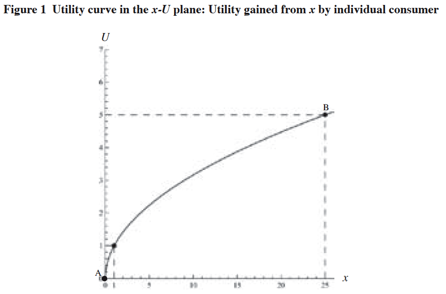
[Notes]
(1) x: Quantity of the composite goods.
(2) U: Utility level of the consumer.
(3) Utility curve: Curve AB.
(4) Utility curve function: ![]()
�y165
�Łz
M >1, and no external economies when M = 0 8�j . From equation (2), we get Figures 2-(a) and (b) to show the utility surface expressed by equation (2) in the x-M-U space. On the other hand, Figure 2-(c) shows a set of iso-utility curves on the utility surface, while Figure 2-(d) shows a set of cross-section curves on
the utility surface cut by x.
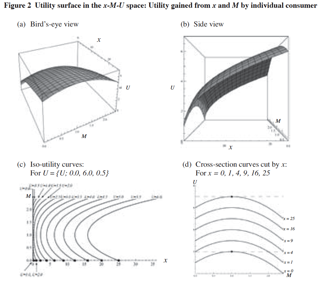
[Notes]
(1) x: Quantity of the composite goods,
M: Equilibrium demand level for the service,
U: Utility level of the consumer.
(2) Utility curve function: 
�y166 �Łz
4�@Equivalent-utility linkage between the utility curve and utility surface
4-1�@Function for the equivalent-utility linkage price
Assume that the income level of a specific consumer is Y, that the unit price of the composite goods is 1.0 which serves as a numéraire9�j , and that the price of the service is P. With the help of this additional assumption, let us try to equalize �gthe utility level of the consumer with income Y who spends all of the income in purchasing the composite goods exclusively�h with �gthe utility level of that consumer which is gained through the consumption of both (��) one unit of the service at price P under the equilibrium demand level M and (��) the composite goods by amount of Y�|P�h as following:
![]()
where Y: Income level of the consumer,
P: Price level of the service,
M: Equilibrium demand level for the service.
Equation (3) can be expressed as

Solving equation (4) for P, we get
![]()
Using equation (5) as the basis, let us set a function g(Y, M) as following:
![]()
Since the value of P in equation (5) indicates the price level of the service that links a point {Y, u0(Y)} in the x�|U plane with a point {Y�|P, M, u1(Y�|P, M)} in the x�|M�|U space, with the condition that u0(Y) = u1(Y�|P, M) 10�j when the income level is Y and the equilibrium demand level is M, we call g(Y, M) in equation (6) the function for the equivalent-utility linkage price (EULP). Under the above framework, the optimization problem which the consumer with income Y has to tackle is described as the issue of maximization over �gthe value of u0(Y) �h and �gthe value of u1(Y�|P, M) subject to the equilibrium demand level M.�h
�@Consequently, with reference to equation (6), if
![]()
,
then, the consumer prefers �gpurchasing one unit of the service and �eY�|P�f amounts of the composite goods�h to �gpurchasing Y amounts of the composite goods exclusively.�h On the other hand, if P �� g(Y, M), then the consumer purchases Y units of the composite goods exclusively. In this context, the EULP function indicates �gthe consumer�fs maximum amount of money that s/he will pay for a unit of the service for given Y and M.�h To assist in understanding the concept of the EULP function, Figure 3 is given as a diagrammatic example for the equation (6) when Y = 25 and M = {M; 0, 1, 0.25} in which it is shown that:
(��) At point A: All the income (Y = 25) is used up for purchasing 25 units of composite goods. The utility level (U) eguals to be 5 in this case.
�y167 �Łz
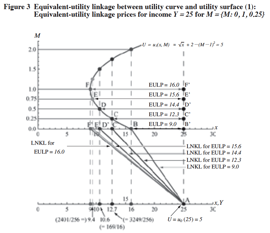
[Notes]
(1) x: Quantity of the composite goods,
M: Equilibrium demand level for the service,
U: Utility level of the consumer,
Y: Income level of the consumer.
(2) EULP: Equivalent-utility linkage price of the service for Y = 25 and M = {M; 0, 1, 0.25}.
This price is expressed by ![]()
(3) Points B, C, D, E and F: Points (x, M) in the x-M plane of the utility surface, which satisfies the condition that u1(x, M) = u0(25) = 5 for M = {M; 0, 1, 0.25}.
(4) Points C�f, D�f, E�f and F�f: Foot of the perpendicular line passing through the points C, D, E and F respectively in the x-M plane.
(5) LNKL: Linkage line which connects point A (on the x-axis of the utility curve) with the point (x, 0) in the x-M plane of the utility surface, which satisfies the condition that u1(x, 0) = u0 (25) = 5 for EULP = 9.0, 12.3, 14.4, 15.6 and 16.0.
(6) Utility curve function: ![]()
(7) Utility surface function: 
(8) Function for the equivalent-utility linkage price (i.e., EULP function) ![]()
(9) Y is equal to x since we set 1.0 for the unit price of the composite goods as a numéraire.
�y168 �Łz
(��) At point B: Given that the equilibrium demand level M is 0 (or�{0), the income is used for purchasing 16 composite goods and one unit of the service (at the price (P) of 9.0) to maintain U = 5. If >9.0, then the consumer purchases 25 composite goods and none of the service at all.
(��) At point C: Given M = 0.25, the income is used for purchasing 12.7 composite goods and one unit of the service (at P = 12.3) to maintain U = 5. If P >12.3, then the consumer purchases 25 composite goods and none of the service at all.
(��) At point D: Given M = 0.5, the income is used for purchasing 10.6 composite goods and one unit of the service (at P = 14.4) to maintain U = 5. If P >14.4, then the consumer purchases 25 composite goods and none of the service at all.
(��) At point E: Given M = 0.75, the income is used for purchasing 9.4 composite goods and one unit the service (at P = 15.6) to maintain U = 5. If P >15.6, then the consumer purchases 25 composite goods and none of the service at all.
(��) At point F: Given M = 1, the income is used for purchasing 9 composite goods and one unit of the service (at P = 16.0) to maintain U = 5. If P >16.0, then the consumer purchases 25 composite goods and none of the service at all.
In the meantime, the surface of the EULP function expressed by equation (6) in the Y-M-P space, is given by Figures 4-(a) �` (c), while Figure 4-(d) exhibits a set of cross-section curves on the surface of the function for the EULP cut by Y. It may be remarked that the cross-section curves of the EULP surface cut by Y shows the bimodal shape with a valley around M = 1 when Y is rather small. This phenomena conflicts with one of our original assumptions that, for any given x, the utility level increases as M moves from 0 to 1 and then starts to decrease thereafter. This fact is somewhat problematic and must be carefully investigated as to why it occurs. However, we will continue to proceed for now with the premise that this problem will not have serious adverse effects upon this paper�fs general approach.
4-2�@Initial linkage price function and maximum linkage price function
If we put M = 0 in equation (6), then we get the function ��(Y) expressed as
![]()
This functional (7) links, for given income level Y, a point on the utility curve with a point which satisfies the condition of M = 0 on the utility surface in such a way that both points remain at the same utility level. We call the function ��(Y) the initial linkage price (ILP) function because it links the two equivalent-utility points, one on the utility curve U = u0(��) and the other on the utility surface U = u1(x, M) with the value of M = 0 which is the initial value12�j of M. For helping us to diagrammatically understand the concept of the ILP function, Figures 5 and 6 are given for the income level Y = 1, 4, 9, 16 and 25 (and 36 in Figure 5), while Figure 7 shows the ILP curve.
�@Similarly, if we put M = 1 in equation (6), then we get the function ��(Y) expressed as
![]()
This function (8) links, for given income level Y, a point on the utility curve with a point which satisfies
�y169 �Łz
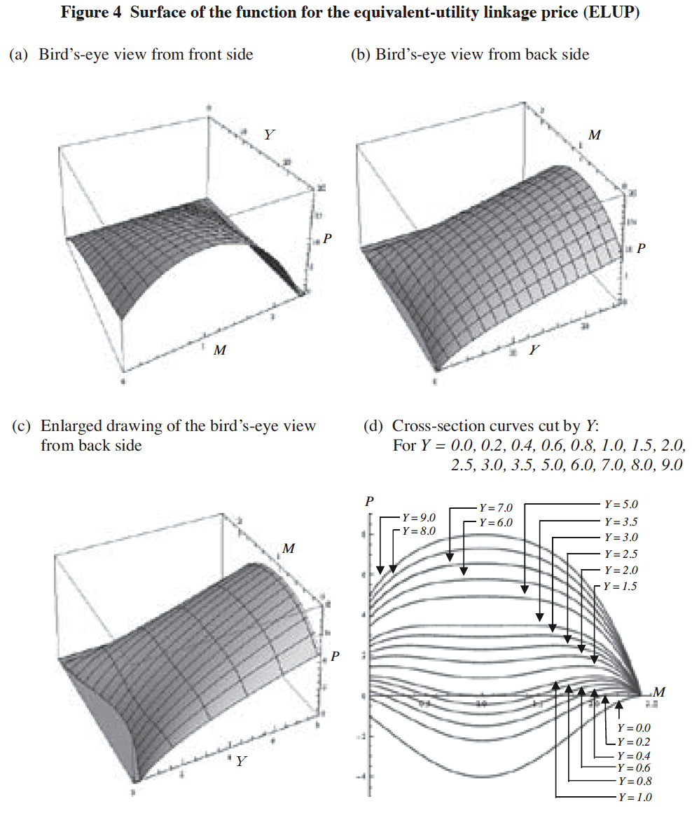
[Notes]
(1) Y: Income level of the consumer,
M: Equilibrium demand level for the service,
P: Price level of the service.
(2) Function for the equivalent-utility linkage price (ELUP): ![]()
(3) Though those curves appearing in the fourth guadrant in Figure 4-(d) are not supposed to exist since we assume P��0 in eguation (3), they are shown as reference.
�y170 �Łz
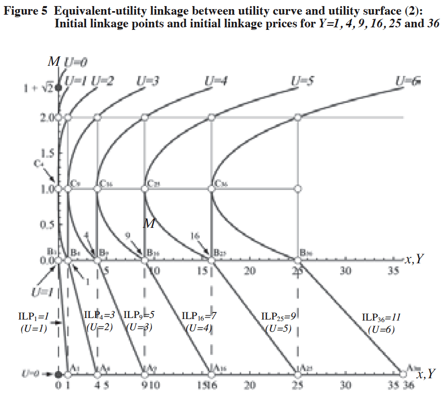
[Notes]
(1) x: Quantity of the composite goods,
M: Equilibrium demand level for the service,
U: Utility level of the consumer,
Y: Income level of the consumer.
(2) Ai: Reference point where x = i on the x-axis of the utility curve U = u0(x).
(3) Bi: Initial linkage point on the x-axis of the utility surface corresponding to its equivalent-utility point Ai (for i = 1, 4, 9, 16, 25, 36).
(4) Ci: Maximum linkage point on the iso-utility curve Bi Ci corresponding to its equivalent-utility point Ai (for i = 1, 4, 9, 16, 25, 36). See Figure 8 for the maximum linkage point.
(5) ILPi: Initial linkage price (ILP) defined as �gthe x-value of point Ai�h subtracted by �gthe x-value of point Bi�h (for i = 1, 4, 9, 16, 25, 36).
(6) Utility curve: ![]()
(7) Utility surface: ![]()
(8) Initial linkage price (ILP) function: ![]()
(9) Y is equal to x on the x-axis of the utility curve U = u0(x) since we set 1.0 for the unit price of x as a numéraire.
�y171 �Łz
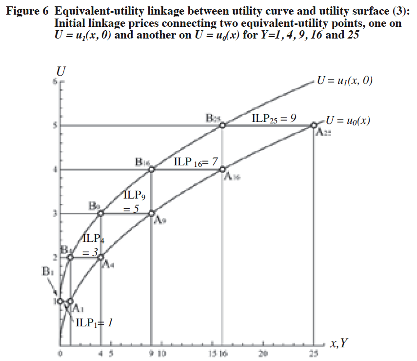
[Notes]
(1) x: Quantity of the composite goods,
U: Utility level of the consumer,
Y: Income level of the consumer.
(2) Ai: Reference point where x = i on the utility curve U = u0(x) (for i = 1, 4, 9, 16, 25).
(3) Bi: Initial linkage point on the curve U = u1(x, 0) corresponding to its equivalent-utility point Ai (for i = 1, 4, 9, 16, 25).
(4) Utility curve of u0(x): ![]()
(5) Utility curve of u1(x, 0): ![]()
(6) ILPi: Initial linkage price (ILP) corresponding to the reference point Ai.
(7) Length of segment ![]() �@ILP25 = 9,
�@ILP25 = 9,
Length of segment ![]() �@ILP16 = 7,
�@ILP16 = 7,
Length of segment ![]() �@ILP9 = 5,
�@ILP9 = 5,
Length of segment ![]() �@ILP4 = 3,
�@ILP4 = 3,
Length of segment ![]() �@ILP1 = 1.
�@ILP1 = 1.
(8) Initial linkage price (ILP) function: ![]()
(9) Y is equal to x on the x-axis of the utility curve U = u0(x) since we set 1.0 for the unit price of x as a numéraire.
�y172 �Łz
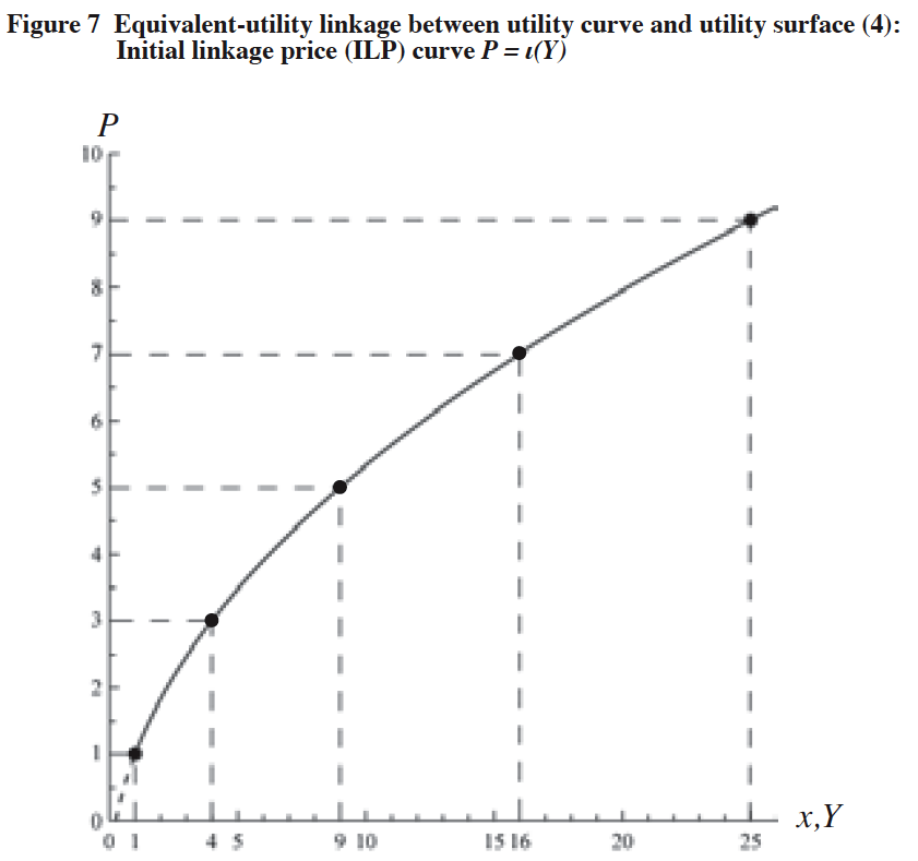
[Notes]
(1) x: Quantity of the composite goods,
Y: Income level of the consumer,
P: Price level of the service.
(2) Initial linkage price (ILP) function: ![]()
(3) Y is equal to x on the x-axis of the utility curve U = u0(x) since we set 1.0 for the unit price of x as a numéraire.
�y173
�Łz
the condition of M = 1 on the utility surface in such a way that both points remain at the same utility level. We call the function ��(Y) the maximum linkage price (MLP) function because it links the two equivalent-utility points, one on the utility curve U = u0(��) and the other on the utility surface U = u1(x, M) with the value of M = 1 which maximizes the utility level of the utility surface for given x. Figure 8 helps us to diagrammatically understand the concept of MLP function for the income level Y = 4, 9, 16 and 25, while Figure 9 shows MLP curve expressed by equation (8).
5�@Density distributions for the income and price
5-1�@Income-density distribution curve
The next task for us is to specify the density distribution function r(Y) over the income level Y of consumers. Along this line, we set:

where Y: Income level of the consumer.
Through the income-density distribution function (9), we assume that the total number of consumers is equal to 2 �~ �gscale-unit of the income Y which is reflected in the income-density distribution function r(Y).�h Figure 10 shows the income-density distribution curve expressed by equation (9).
5-2�@Price-density distribution surface
If we transform, through the EULP function P = g(Y, M) expressed by equation (6), the incomedensity distribution function r(Y) expressed by equation (9) into the density distribution function over the price P of the service, then we gain the price-density distribution function s(M, P) expressed by

The price-density distribution function s(M, P) can be obtained by means of the following transformation of the income-density distribution function r(Y):
![]()
In case s(M, P) contains Y in equation (11), we substitute g�|1(P, M) for Y.
Figures 11-(a) ~ (d) shows the price-density distribution surface expressed by equation (11). In addition, Figure 11-(e) shows the price-density distribution curve expressed by s(0, P) and s(2, P), while Figure-(f) shows the price-density distribution curve expressed by s(1, P).
6�@Demand surface
6-1�@Demand surface function
From equation (10), we obtain the demand surface (DS)13�j function h(N,M) by the following way. First, we set

where N: Demand level of the service at price level P under given M,
�y174 �Łz
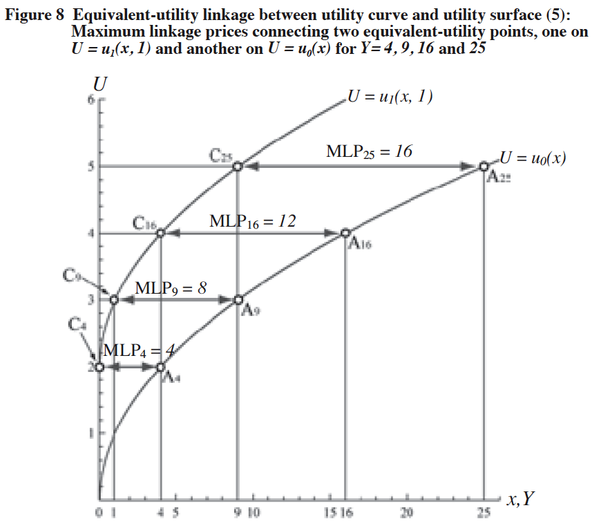
[Notes]
(1) x: Quantity of the composite goods,
U: Utility level of the consumer,
Y: Income level of the consumer.
(2) Ai: Reference point where x = i on the utility curve U = u0(x) (for i = 1, 4, 9, 16, 25).
(3) Ci: Maximum linkage point on the curve U=u1(x, 1) corresponding to its equivalent-utility point Ai (for i = 1, 4, 9, 16, 25).
(4) Utility curve of u0(x): ![]()
(5) Utility curve of u1(x, 0): ![]()
(6) MLPi: Maximum linkage price (MLP) corresponding to the reference point A.
(7) Length of segment ![]() �@MLP25 = 16,
�@MLP25 = 16,
Length of segment ![]() �@MLP16 = 12,
�@MLP16 = 12,
Length of segment ![]() �@MLP9 = 8,
�@MLP9 = 8,
Length of segment ![]() �@MLP4 = 4,
�@MLP4 = 4,
(8) Maximum linkage price (MLP) function: ![]()
(9) Y is equal to x on the x-axis of the utility curve U = u0(x) since we set 1.0 for the unit price of x as a numéraire.
�y175 �Łz
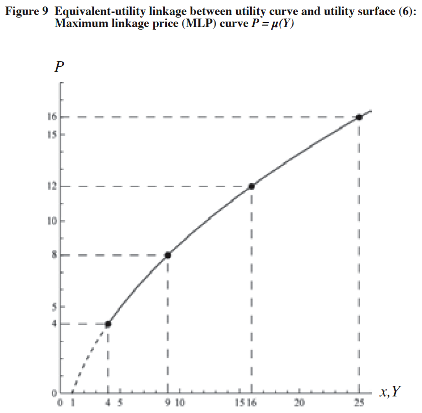
[Notes]
(1) x: Quantity of the composite goods,
Y: Income level of the consumer,
P: Price level of the service.
(2) Maximum linkage price (MLP) function: ![]()
(3) Y is equal to x on the x-axis of the utility curve U = u0(x) since we set 1.0 for the unit price of x as a numéraire.
�y176 �Łz
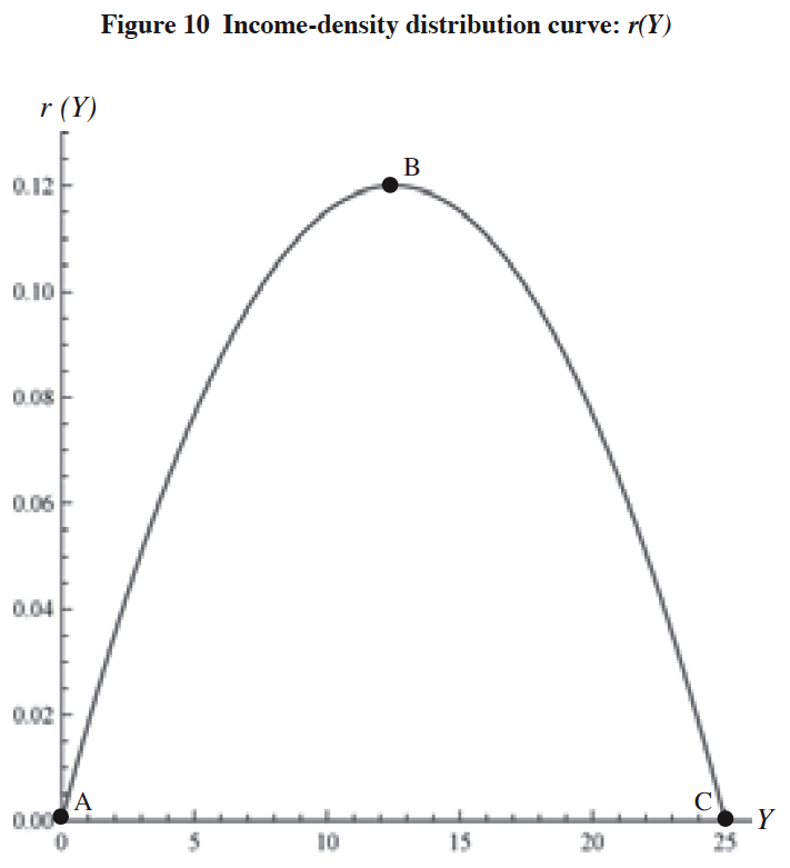
[Notes]
(1) Y: Income level of the consumer.
(2) Income-density distribution function r(Y): 
(3) Income-density distribution curve: Curve ABC.
(4) Coordinate values of point B: Y = 12.5, r(Y) = 0.12.
(5) 
(6) This implies that the total number of consumers is equal to 2 �~ �gscale-unit of the income level Y which is reflected in the income-density distribution function r(Y).�h
�y177 �Łz
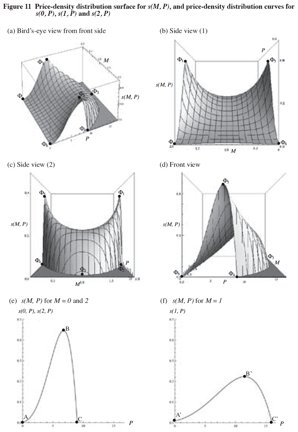
�y178 �Łz
[Notes]
(1) M: Equilibrium demand level for the service,
P: Price level of the service.
(2) s(M, P): Price-density distribution function 
(3) Price-density distribution surface: Surface ����1��2��3��4��5.
(4) s(M, P) for M=0 and 2:s(0, P) = s(2, P) = —(3(-9+P)(1+P)3 (11+P))/125000 �@�@for 0��P��9.
(5) Coordinate values of point B: P ≐ 6.7460, s(0, P) = s(2, P) ≐ 0.4462.
(6) s(M, P) for M =1: s(1, P) = —(3(-16+P) (4+P)3 (24+P))/8000000�@�@�@�@�@�@for 0��P��16.
(7) Coordinate values of point B�f: P ≐ 11.4919, s(1, P) ≐ 0.2231.
(8) 
(9) 
(10) Total number of consumers: 2 �~ �gscale-unit of the income level Y which is reflected in the income-density distribution function r(Y).�h
M:�@�@ �@�@�@Equilibrium demand level for the service,
P: �@�@�@ �@�@Price level of the service,
s(M, P): �@�@Price-density distribution function,
PMAX(M): The value of P which is obtained by substituting 2514�j for Y in the EULP function (6).
Then, by solving the equation (12) for P, we obtain the DS function expressed by
�@(13) P = h(N, M).
The equation (13) can be expressed in the form of implicit function for P as
�@((11+(-2+M)M(-12+(-2+M)M)+P)2(-9+(-2+M)M(8+(-2+M)M)+P)2((-1+(-2+M)M)2(51+M(4+M(2+(-4+M)M)))+2(-1+(-2+M)M) P+P2))/(250000((-1+(-2+M)M)6) = N.
Its explicit functional expression of the DS is given in Appendix A-(1)15�j .
�@Based on this result, we get Figure 12 where the DS in the N-M-P space expressed by equation (13) is illustrated in Figures 12-(a) ~ (c), while a set of cross-section curves of the DS cut by M is shown in Figure 12-(d) and that cut by N in Figure 12-(e).
6-2�@Basic characteristics of the shape of demand surface
As can be seen from Figure 12, the DS has the following characteristics.
�y179 �Łz
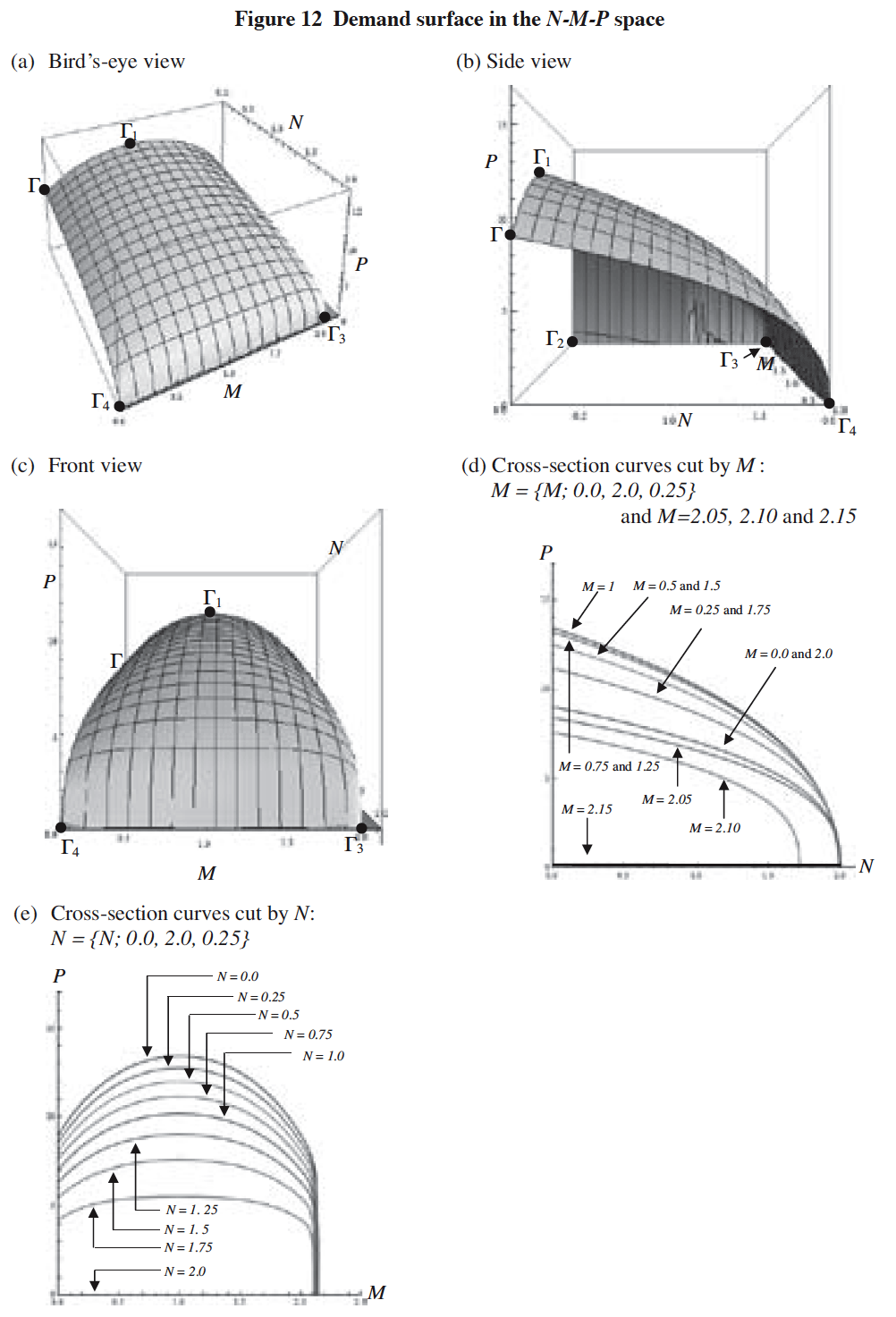
�y180 �Łz
[Notes]
(1) N: Demand level for the service (i.e., the number of consumers who demand the service at price P under the condition of given M),
M: Equilibrium demand level for the service,
P: Price level of the service.
(2) Demand surface: Surface ����1��2��3��4
(3) Demand surface (DS) function: P = h(N, M)
(i) In the form of implicit function for P:
((11+(-2+M)M(-12+(-2+M)M)+P)2(-9+(-2+M)M(8+(-2+M)M)+P)2((-1+(-2+M)M)2 (51+M(4+M(2+(-4+M)M)))+2(-1+(-2+M)M)2P+P))/(250000(-1+(-2+M)M)6) = N.
(ii) In the form of explicit function for P: P = h(N, M) = as given in Appendix A-(1).
(4) Total number of consumers: 2 �~ �gscale-unit of N.�h
(��) Figures 12-(a) �` (c) show that the shape of the DS resembles a platypus�f upper bill with its right-hand side vertically trimmed to a degree.
(��) Figure 12-(d) shows that the height of the cross-section curve of the DS cut by M in this figure, increases as M approaches to 1 from 0, and then decreases as M rises from M = 1. This implies that there exist T-external economies centering around M =1 and that the price elasticity of the cross-section curve at a point for given N increases as the curve recedes from M = 1 to its lower and higher values.
(��) Figure 12-(e) shows that any of the cross-section curves of the DS cut by N in this figure, has upward convexity and forms a bell-shaped curve with its vertex at M = 1, while the height of the cross-section curve decreases as N increases.
7�@Quasi-derived demand curve and derived demand curve
7-1�@Quasi-derived demand curve function
Once we have obtained the DS, the next question is how to obtain the actual market demand curve from the DS. To deal with this enquiry, let us draw the curve ������ on the demand surface as shown in Figures 13-(a) and (b), which is the locus of the points that satisfy the following two requirements:
(��) The point is situated on the demand surface.
(��) The point satisfies the condition N = M after adjustment of the scale-unit of M to that of N.
We understand that any point on the curve ������ that meets a given price surface in the N-M-P space can become an actual market equilibrium point. That is to say, the curve ������ is the actual demand curve expressed in the three-dimensional N-M-P space. We therefore call this curve the quasi-derived demand (QDD) curve because this curve is derived at one step before obtaining the derived demand curve which is expressed in the two-dimensional N-P plane which we discuss in the next sub-section.
�y181 �Łz
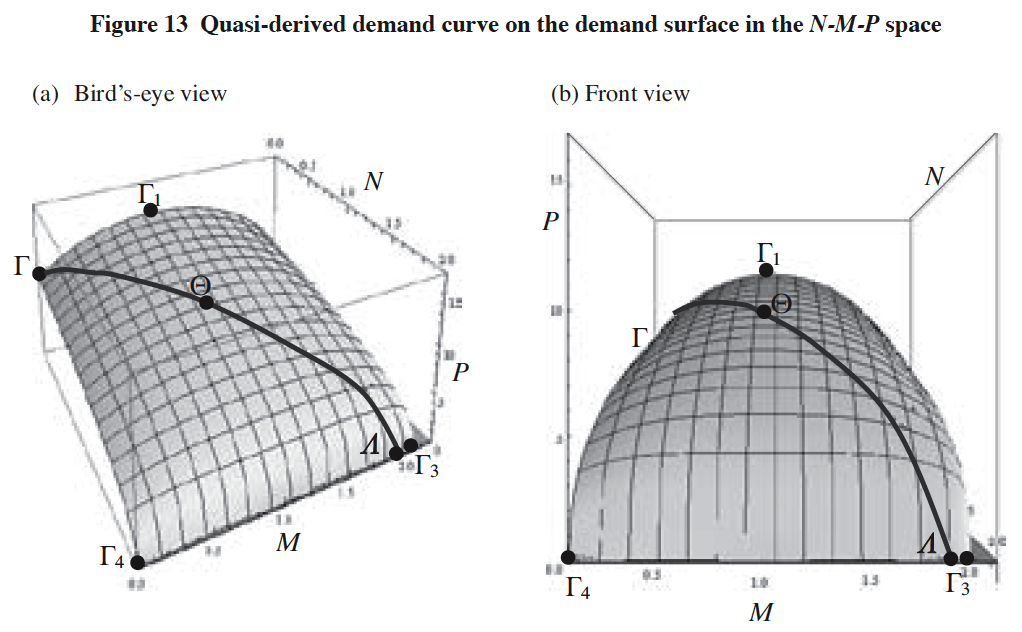
[Notes]
(1) N: Demand level for the service
M: Equilibrium demand level for the service,
P: Price level of the service.
(2) Demand surface: Surface ����1��3��4.
(3) Demand surface (DS) function: P = h(N, M)
(i) In the form of implicit function for P:
((11+(-2+M)M(-12+(-2+M)M)+P)2(-9+(-2+M)M(8+(-2+M)M)+P)2((-1+(-2+M)M)2 (51+M(4+M(2+(-4+M)M)))+2(-1+(-2+M)M)P+P2))/(250000(-1+(-2+M)M)6) = N.
(ii) In the form of explicit function for P: P = h(N, M) = as given in Appendix A-(1).
(4) Total number of consumers: 2 �~ �gscale-unit of N.�h
(5) Quasi-derived demand (QDD) curve: Curve ������.
The QDD curve in the N-M-P space is the locus of the point (i) that is situated on the demand surface and (ii) that satisfies the condition of M = N after adjustment of the scale-unit of M to that of N.
�y182 �Łz
7-2�@Derived demand curve function
If we make the orthographic projection of the QDD curve in the N-M-P space onto the N-P plane, then we obtain the curve ABC as shown in Figure 14. Since this curve is derived from the demand surface and since it shows the actual market demand, we call it the derived demand (DD)16�j curve. The DD function DD(N) can be gained by replacing N for M in the DS function h(N,M) as
�@(14) P = DD(N) = h(N, N)
�@�@�@where N: Demand level for the service.
It will be noted that the DD curve exhibits a bell-shaped form. From Appendix A-(1) and equation (14),�@we obtain the DD curve function whose explicit functional expression for equation (14) is given in Appendix A-(2).
7-3�@Equilibrium points on the derived demand curve
After having obtained the DD curve, let us introduce a price function P(N)17�j to note the following as to the stability of the equilibrium point Ne which is defined as a point of intersection of the price curve with the derived demand (DD) curve where the condition P(Ne) = DD(Ne) is satisfied in the N-P plane.
(��) In case when the price curve crosses the DD curve at two different points, the left-hand intersection where the price curve cuts the DD curve from above to below is the unstable equilibrium point, while the right-hand intersection where the price curve cuts the DD curve from below to above is the stable equilibrium point.
(��) In case when the price curve is tangent to the DD curve from above, the point of contact of the two curves is �gthe quasi-stable point toward the right�h in the sense that if the demand level infinitesimally increases (i.e., infinitesimally moves to rightward) from this quasistable point, then the demand level tends to turn back to the original point, but that if the demand level decreases even infinitesimally (i.e., even infinitesimally moves to leftward) from this quasi-stable point, then the demand level starts to decrease furthermore.
(��) In case when the price curve is tangent to the DD curve from below18�j , the point of contact of the two curves is �gthe quasi-stable point toward the left�h in the sense that if the demand level infinitesimally decreases (i.e., infinitesimally moves to leftward) from this quasi-stable point, then the demand level tends to turn back to the original point, but that if the demand level increases even infinitesimally (i.e., even infinitesimally moves to rightward) from this quasi-stable point, then the demand level starts to increase furthermore.
8�@Conclusion: Agenda for further work
We have in this paper initiated the attempt to mathematically obtain the demand surface from a set of a utility curve, a utility surface which reflects the existence of the T-external economies, and an income-
�y183 �Łz
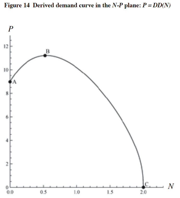
[Notes]
(1) N: Demand level for the service,
P: Price level of the service.
(2) Derived demand (DD) curve: Curve ABC.
This bell-shaped curve is obtained through the orthographic projection of the quasi-derived demand (QDD) curve in the N-M-P space onto the N-P plane.
(3) Coordinate values of point A: N = 0.0, �@�@�@�@�@�@�@�@P = 9,
Coordinate values of point B (vertex): N ≐0.5440, �@P ≐ 11.2043,
Coordinate values of point C: N ≐ 1.9992 ≐ 2.0, �@ P= 0.0.
(4) Derived demand (DD) function P = DD(N):
(i) In the form of implicit function for P:
((11+(-2+N)N(-12+(-2+N)N)+P)2(-9+(-2+N)N(8+(-2+N)N)+P)2((-1+(-2+N)N)2 (51+N(4+N(2+(-4+N)N)))+2(-1+(-2+N)N2)P+P2 ))-N/(250000(-1+(-2+N)N)6) = 0.
(ii) In the form of explicit function for P: P = DD(N) = as given in Appendix A-(2).
�y184
�Łz
density distribution curve. Our obtained demand surface is presumably not perfect yet, and there is much remaining to be done for refining the approach applied in this paper. A more in-depth investigation is necessary to identify the effects of the following phenomena on the ultimate shape of the resulting demand surface:
(��) The cross-section curves of the equivalent-utility linkage price (EULP) surface cut by Y have the bimodal shapes when the level of Y is relatively small, that is, when the level of Y is approximately less than 2.0. [Figure 4]
(��) The initial linkage price (ILP) curve does not exist when the level of Y is less than 1.0. [Figure 7]
(��) The maximum linkage price (MLP) curve does not exist when the level of Y is less than 4.0. [Figure 9]
(��) The price-density distribution curve for M = 1 has the positive value when the price level of the service is 0.0. [Figure 11-(f)]
(��) There exists a disorderly layout of zigzag lines drawn by Mathematica on the directly opposite inside-wall of the demand surface. [Figure 12-(b)]
Meanwhile, among other research works that we want to carry out in the near future are as following.
(��) To search for an initial set of the utility curve, utility surface and income-density distribution curve which would enable us to obtain the semidome-shaped demand surface as dealt with in Kawashima et al. (2007).
(��) To find an initial set of the utility curve, utility surface and income-density distribution curve which provides us with the less-steep right edge of the cross-section curves of the demand surface cut by M. [Figure 12-(d)]
(��) To examine what kind of shape of the demand surface we obtain if we initially employ the utility surface expressed by ![]()
(��) To make it sure whether we can obtain the demand surface19�j which is neutral to the T-external economies if we employ the utility surface expressed by the function which is
neutral to the T-external economies such as ![]()
(��) To obtain, from the demand surface function, the gross social benefit (GSB) (i.e., gross consumer�fs surplus) function and the marginal social benefit (MSB) (i.e., marginal consumer�fs surplus) function to discuss, for given marginal social cost function, the optimum demand level for the service. In conjunction with this, the GSB function GSB(N) for the demand level N is formulated as
�@
while the MSB function MSB(N) for the demand level N is expressed by
�y185 �Łz
�@
�@where N: Demand level for the service,
M: Equilibrium demand level for the service,
h(N, M): Demand surface function.
Our attempt has not necessarily generated fully conclusive results and some items mentioned in the above research agenda are more or less mathematically intractable. The authors hope, however, that the theoretical endeavor of this paper has made one step forward trekking along the route of the demand surface to shed new light upon the analytical concept of external agglomeration economies, and that some of our fellow trekkers may join the authors in a scientific exploration to scale and map the heights and configuration of the T-external economies.
References
[1] Buchanan, J.M., 1965, �gAn Economic Theory of Clubs,�h Economica, 32(125), pp.1-14.
[2] Kawashima, T., 1975, �gEconomics of Urban Environments: Diagrammatic Analysis,�h Shin Toshi, Vol.29, No.3, Toshi Keikaku Kyokai, Tokyo, pp. 4-14 (in Japanese).
[3] Kawashima, T., N. Hiraoka, J. Noro and R. Samata, 2007, �gExternal Economies (Demand Surface Analysis�qNo.1�r): Derived Demand Curve and Marginal Social Benefit Curve Obtained from the Demand Surface,�h Gakushuin Economic Papers, Vol.44, No.3, Gakushuin University, Tokyo, pp.203-262 (in Japanese).
[4] Kawashima, T. and J. Noro, 2010, �gExternal Economies (Demand Surface Analysis�qNo.4�r): Bendback Demand Curve and Its Corresponding Marginal Social Benefit Curve, and Optimum Levels of Taxes and Subsidies to Maximize the Net Social Benefit,�h Gakushuin Economic Papers, Vol.46, No.3-4, Gakushuin University, Tokyo, pp.1-30 (in Japanese).
[5] Leibenstein, H., 1950, �gBandwagon, Snob and Veblen Effects in the Theory of Consumers’ Demand,�h The Quarterly Journal of Economics, Vol.64, No.2, pp.183-207.
[6] Noro, J., T. Kawashima, and N. Hiraoka, 2009, �gExternal Economies (Demand Surface Analysis �qNo.2�r): Maximization of Net Social Benefit (Optimum Levels of Demands, Taxes and Subsidies)�h Gakushuin Economic Papers, Vol.46, No.1, Gakushuin University, Tokyo, pp.31-67 (in Japanese).
[7] Noro, J. and T. Kawashima, 2009, �gExternal Economies (Demand Surface Analysis�qNo.3�r): Optimum Level of Scholarship to be granted to the Students who participate in the University NGO Volunteer Activity Programme,�h Gakushuin Economic Papers, Vol.46, No.2, Gakushuin University, Tokyo, pp.171-186 (in Japanese).
�y186 �Łz
Appendix A-(1)
Demand surface function:P = h(N, M) =-(0.333333 (-0.00354 - 0.04224 M - 0.18816 M^2 - 0.33984 M^3 - 0.02544 M^4 + 0.59808 M^5 + 0.20976
M^6 - 0.63072 M^7 + 0.01932 M^8 + 0.38592 M^9 - 0.25824 M^10 + 0.04992 M^11 + 0.02496 M^12 - 0.02016 M^13 + 0.00624 M^14 - 0.00096 M^15 + 0.00006 M^16))/(-0.00232 -
0.01824 M - 0.04368 M^2 - 0.0112 M^3 + 0.0636 M^4 + 0.00576 M^5 - 0.05408 M^6 + 0.03264 M^7 - 0.0012 M^8 - 0.008 M^9 + 0.00432 M^10 - 0.00096 M^11 + 0.00008 M^12) -
(0.419974 (4.00536*10^-6 + 0.0000948787 M + 0.000978762 M^2 + 0.00566415 M^3 + 0.0194244 M^4 + 0.0361034 M^5 + 0.0149257 M^6 - 0.0759965 M^7 - 0.121993 M^8 + 0.0544458
M^9 + 0.236258 M^10 - 0.0178633 M^11 - 0.311927 M^12 + 0.0464877 M^13 + 0.311695 M^14 - 0.144165 M^15 - 0.19215 M^16 + 0.198096 M^17 + 0.0090106 M^18 - 0.112272 M^19 +
0.0686945 M^20 - 0.00327253 M^21 - 0.0187682 M^22 + 0.0126184 M^23 - 0.00389038 M^24 + 0.000242012 M^25 + 0.000334495 M^26 - 0.000174505 M^27 + 0.0000483264 M^28 -
8.64*10^-6 M^29 + 1.00224*10^-6 M^30 - 6.912*10^-8 M^31 + 2.16*10^-9 M^32))/((-0.00232 - 0.01824 M - 0.04368 M^2 - 0.0112 M^3 + 0.0636 M^4 + 0.00576 M^5 - 0.05408 M^6 +
0.03264 M^7 - 0.0012 M^8 - 0.008 M^9 + 0.00432 M^10 - 0.00096 M^11 + 0.00008 M^12) (-0.00029065 - 0.00805802 M - 0.099448 M^2 - 0.711633 M^3 - 3.19793 M^4 - 8.94484 M^5 -
13.246 M^6 + 0.394776 M^7 + 37.4862 M^8 + 45.9321 M^9 - 34.9084 M^10 - 104.846 M^11 + 11.6718 M^12 + 149.55 M^13 - 5.97507 M^14 - 167.343 M^15 + 40.3348 M^16 + 140.279
M^17 - 89.2752 M^18 - 62.0906 M^19 + 93.3987 M^20 - 18.0172 M^21 - 38.3905 M^22 + 33.8874 M^23 - 7.57329 M^24 - 6.25114 M^25 + 6.0458 M^26 - 2.19781 M^27 + 0.0958468
M^28 + 0.299809 M^29 - 0.174684 M^30 + 0.0631529 M^31 - 0.0203024 M^32 + 0.00600624 M^33 - 0.000706328 M^34 - 0.00073857 M^35 + 0.000617074 M^36 - 0.000255983 M^37 +
0.0000623877 M^38 - 4.96101*10^-6 M^39 - 2.95538*10^-6 M^40 + 1.58591*10^-6 M^41- 4.48954*10^-7M^42 + 8.80451*10^-8 M^43 - 1.25888*10^-8 M^44 + 1.3036*10^-9 M^45 -
9.3312*10^-11 M^46 + 4.1472*10^-12 M^47 - 8.64*10^-14 M^48 + 0.000145325 N + 0.004029 M N + 0.0497239 M^2 N + 0.355815 M^3 N + 1.59896 M^4 N + 4.47237 M^5 N + 6.62283
M^6 N - 0.197838 M^7 N - 18.7438 M^8 N - 22.9662 M^9 N + 17.4562 M^10 N + 52.4269 M^11 N - 5.83572 M^12 N -74.7833 M^13 N + 2.97929 M^14 N + 83.6816 M^15 N - 20.1476
M^16 N - 70.1471 M^17 N + 44.6068 M^18 N + 31.0508 M^19 N - 46.6613 M^20 N + 9.00075 M^21 N + 19.1566 M^22 N - 16.9283 M^23 N + 3.81644 M^24 N + 3.10305 M^25 N -
3.03621 M^26 N + 1.12011 M^27 N - 0.0500609 M^28 N - 0.160729 M^29 N + 0.0945976 M^30 N - 0.0309713 M^31 N + 0.0067843 M^32 N - 0.00102228 M^33 N + 0.000102643 M^34 N
- 6.2208*10^-6 M^35 N +1.728*10^-7 M^36 N + [Sqrt](4. (4.00536*10^-6 + 0.0000948787 M + 0.000978762 M^2 + 0.00566415 M^3 + 0.0194244 M^4 + 0.0361034 M^5 + 0.0149257 M^6
- 0.0759965 M^7 - 0.121993 M^8 + 0.0544458 M^9 + 0.236258 M^10 - 0.0178633 M^11 - 0.311927 M^12 + 0.0464877 M^13 + 0.311695 M^14 - 0.144165 M^15 - 0.19215 M^16 + 0.198096
M^17 + 0.0090106 M^18 - 0.112272 M^19 + 0.0686945 M^20 - 0.00327253 M^21 - 0.0187682 M^22 + 0.0126184 M^23 - 0.00389038 M^24 + 0.000242012 M^25 + 0.000334495 M^26 -
0.000174505 M^27 + 0.0000483264 M^28 - 8.64*10^-6 M^29 + 1.00224*10^-6 M^30 - 6.912*10^-8 M^31 + 2.16*10^-9 M^32)^3 + (-0.00029065 - 0.00805802 M - 0.099448 M^2 -
0.711633 M^3 - 3.19793 M^4 - 8.94484 M^5 - 13.246 M^6 + 0.394776 M^7 + 37.4862 M^8 + 45.9321 M^9 - 34.9084 M^10 - 104.846 M^11 + 11.6718 M^12 + 149.55 M^13 - 5.97507 M^14
- 167.343 M^15 + 40.3348 M^16 + 140.279 M^17 - 89.2752 M^18 - 62.0906 M^19 + 93.3987 M^20 - 18.0172 M^21 - 38.3905 M^22 + 33.8874 M^23 - 7.57329 M^24 - 6.25114 M^25 +
6.0458 M^26 - 2.19781 M^27 + 0.0958468 M^28 + 0.299809 M^29 - 0.174684 M^30 + 0.0631529 M^31 - 0.0203024 M^32 + 0.00600624 M^33 - 0.000706328 M^34 - 0.00073857 M^35 +
0.000617074 M^36 - 0.000255983 M^37 + 0.0000623877 M^38 - 4.96101*10^-6 M^39 - 2.95538*10^-6 M^40 + 1.58591*10^-6 M^41 - 4.48954*10^-7 M^42 + 8.80451*10^-8 M^43 -
1.25888*10^-8 M^44 + 1.3036*10^-9 M^45 - 9.3312*10^-11 M^46 + 4.1472*10^-12 M^47 - 8.64*10^-14 M^48 + 0.000145325 N + 0.004029 M N + 0.0497239 M^2 N + 0.355815 M^3 N +
1.59896 M^4 N + 4.47237 M^5 N + 6.62283 M^6 N - 0.197838 M^7 N - 18.7438 M^8 N - 22.9662 M^9 N + 17.4562 M^10 N + 52.4269 M^11 N - 5.83572 M^12 N - 74.7833 M^13 N +
2.97929 M^14 N + 83.6816 M^15 N - 20.1476 M^16 N - 70.1471 M^17 N + 44.6068 M^18 N + 31.0508 M^19 N - 46.6613 M^20 N + 9.00075 M^21 N + 19.1566 M^22 N - 16.9283 M^23 N
+ 3.81644 M^24 N + 3.10305 M^25 N - 3.03621 M^26 N + 1.12011 M^27 N - 0.0500609 M^28 N - 0.160729 M^29 N + 0.0945976 M^30 N - 0.0309713 M^31 N + 0.0067843 M^32 N -
0.00102228 M^33 N + 0.000102643 M^34 N - 6.2208*10^-6 M^35 N +1.728*10^-7 M^36 N)^2))^(1/3)) + (0.264567 (-0.00029065 - 0.00805802 M - 0.099448 M^2 - 0.711633 M^3 -
3.19793 M^4 - 8.94484 M^5 - 13.246 M^6 + 0.394776 M^7 + 37.4862 M^8 + 45.9321 M^9 - 34.9084 M^10 - 104.846 M^11 + 11.6718 M^12 + 149.55 M^13 - 5.97507 M^14 - 167.343 M^15
+ 40.3348 M^16 + 140.279 M^17 - 89.2752 M^18 - 62.0906 M^19 + 93.3987 M^20 - 18.0172 M^21 - 38.3905 M^22 + 33.8874 M^23 - 7.57329 M^24 - 6.25114 M^25 + 6.0458 M^26 -
2.19781 M^27 + 0.0958468 M^28 + 0.299809 M^29 - 0.174684 M^30 + 0.0631529 M^31 - 0.0203024 M^32 + 0.00600624 M^33 - 0.000706328 M^34 - 0.00073857 M^35 + 0.000617074
M^36 - 0.000255983 M^37 + 0.0000623877 M^38 - 4.96101*10^-6 M^39 - 2.95538*10^-6 M^40 + 1.58591*10^-6 M^41 - 4.48954*10^-7 M^42 + 8.80451*10^-8 M^43 - 1.25888*10^-8
M^44 + 1.3036*10^-9 M^45 - 9.3312*10^-11 M^46 + 4.1472*10^-12 M^47 - 8.64*10^-14 M^48 + 0.000145325 N + 0.004029 M N + 0.0497239 M^2 N + 0.355815 M^3 N + 1.59896 M^4 N
+ 4.47237 M^5 N + 6.62283 M^6 N - 0.197838 M^7 N - 18.7438 M^8 N - 22.9662 M^9 N + 17.4562 M^10 N + 52.4269 M^11 N - 5.83572 M^12 N - 74.7833 M^13 N + 2.97929 M^14 N +
83.6816 M^15 N - 20.1476 M^16 N - 70.1471 M^17 N + 44.6068 M^18 N + 31.0508 M^19 N - 46.6613 M^20 N + 9.00075 M^21 N + 19.1566 M^22 N - 16.9283 M^23 N + 3.81644 M^24 N
+ 3.10305 M^25 N - 3.03621 M^26 N + 1.12011 M^27 N - 0.0500609 M^28 N - 0.160729 M^29 N + 0.0945976 M^30 N - 0.0309713 M^31 N + 0.0067843 M^32 N - 0.00102228 M^33 N +
0.000102643 M^34 N - 6.2208*10^-6 M^35 N + 1.728*10^-7 M^36 N + \[Sqrt](4. (4.00536*10^-6 + 0.0000948787 M + 0.000978762 M^2 + 0.00566415 M^3 + 0.0194244 M^4 + 0.0361034
M^5 + 0.0149257 M^6 - 0.0759965 M^7 - 0.121993 M^8 + 0.0544458 M^9 + 0.236258 M^10 - 0.0178633 M^11 - 0.311927 M^12 + 0.0464877 M^13 + 0.311695 M^14 - 0.144165 M^15 -
0.19215 M^16 + 0.198096 M^17 + 0.0090106 M^18 - 0.112272 M^19 + 0.0686945 M^20 - 0.00327253 M^21 - 0.0187682 M^22 + 0.0126184 M^23 - 0.00389038 M^24 + 0.000242012 M^25
+ 0.000334495 M^26 - 0.000174505 M^27 + 0.0000483264 M^28 - 8.64*10^-6 M^29 + 1.00224*10^-6 M^30 - 6.912*10^-8 M^31 + 2.16*10^-9 M^32)^3 + (-0.00029065 - 0.00805802 M -
0.099448 M^2 - 0.711633 M^3 - 3.19793 M^4 - 8.94484 M^5 - 13.246 M^6 + 0.394776 M^7 + 37.4862 M^8 + 45.9321 M^9 - 34.9084 M^10 - 104.846 M^11 + 11.6718 M^12 + 149.55 M^13
- 5.97507 M^14 - 167.343 M^15 + 40.3348 M^16 + 140.279 M^17 - 89.2752 M^18 - 62.0906 M^19 + 93.3987 M^20 - 18.0172 M^21 - 38.3905 M^22 + 33.8874 M^23 - 7.57329 M^24 -
6.25114 M^25 + 6.0458 M^26 - 2.19781 M^27 + 0.0958468 M^28 + 0.299809 M^29 - 0.174684 M^30 + 0.0631529 M^31 - 0.0203024 M^32 + 0.00600624 M^33 - 0.000706328 M^34 -
0.00073857 M^35 + 0.000617074 M^36 - 0.000255983 M^37 + 0.0000623877 M^38 - 4.96101*10^-6 M^39 - 2.95538*10^-6 M^40 + 1.58591*10^-6 M^41 - 4.48954*10^-7 M^42 +
8.80451*10^-8 M^43 - 1.25888*10^-8 M^44 + 1.3036*10^-9 M^45 - 9.3312*10^-11 M^46 + 4.1472*10^-12 M^47 - 8.64*10^-14 M^48 + 0.000145325 N + 0.004029 M N + 0.0497239 M^2
N + 0.355815 M^3 N + 1.59896 M^4 N + 4.47237 M^5 N + 6.62283 M^6 N - 0.197838 M^7 N - 18.7438 M^8 N - 22.9662 M^9 N + 17.4562 M^10 N + 52.4269 M^11 N - 5.83572 M^12 N -
74.7833 M^13 N + 2.97929 M^14 N + 83.6816 M^15 N - 20.1476 M^16 N - 70.1471 M^17 N + 44.6068 M^18 N + 31.0508 M^19 N - 46.6613 M^20 N + 9.00075 M^21 N + 19.1566 M^22 N
- 16.9283 M^23 N + 3.81644 M^24 N + 3.10305 M^25 N - 3.03621 M^26 N + 1.12011 M^27 N - 0.0500609 M^28 N - 0.160729 M^29 N + 0.0945976 M^30 N - 0.0309713 M^31 N +
0.0067843 M^32 N - 0.00102228 M^33 N + 0.000102643 M^34 N - 6.2208*10^-6 M^35 N + 1.728*10^-7 M^36 N)^2))^(1/3))/(-0.00232 - 0.01824 M - 0.04368 M^2 - 0.0112 M^3 + 0.0636
M^4 + 0.00576 M^5 - 0.05408 M^6 + 0.03264 M^7 - 0.0012 M^8 - 0.008 M^9 + 0.00432 M^10 - 0.00096 M^11 + 0.00008 M^12).
Appendix A-(2)
Derived demandcurve function: P = DD(N) =-(0.333333 (-0.00354 - 0.04224 N - 0.18816 N^2 - 0.33984 N^3 - 0.02544 N^4 + 0.59808 N^5 +
0.20976 N^6 - 0.63072 N^7 + 0.01932 N^8 + 0.38592 N^9 - 0.25824 N^10 + 0.04992 N^11 + 0.02496 N^12 - 0.02016 N^13 + 0.00624 N^14 - 0.00096 N^15 + 0.00006 N^16))/(-0.00232 -
0.01824 N - 0.04368 N^2 - 0.0112 N^3 + 0.0636 N^4 + 0.00576 N^5 - 0.05408 N^6 + 0.03264 N^7 - 0.0012 N^8 - 0.008 N^9 + 0.00432 N^10 - 0.00096 N^11 + 0.00008 N^12) - (0.419974
(4.00536*10^-6 + 0.0000948787 N + 0.000978762 N^2 + 0.00566415 N^3 + 0.0194244 N^4 + 0.0361034 N^5 + 0.0149257 N^6 - 0.0759965 N^7 - 0.121993 N^8 + 0.0544458 N^9 +
0.236258 N^10 - 0.0178633 N^11 - 0.311927 N^12 + 0.0464877 N^13 + 0.311695 N^14 - 0.144165 N^15 - 0.19215 N^16 + 0.198096 N^17 + 0.0090106 N^18 - 0.112272 N^19 + 0.0686945
N^20 - 0.00327253 N^21 - 0.0187682 N^22 + 0.0126184 N^23 - 0.00389038 N^24 + 0.000242012 N^25 + 0.000334495 N^26 - 0.000174505 N^27 + 0.0000483264 N^28 - 8.64*10^-6 N^29
+ 1.00224*10^-6 N^30 - 6.912*10^-8 N^31 + 2.16*10^-9 N^32))/((-0.00232 - 0.01824 N - 0.04368 N^2 - 0.0112 N^3 + 0.0636 N^4 + 0.00576 N^5 - 0.05408 N^6 + 0.03264 N^7 - 0.0012 N^8
- 0.008 N^9 + 0.00432 N^10 - 0.00096 N^11 + 0.00008 N^12) (-0.00029065 - 0.0079127 N - 0.095419 N^2 - 0.661909 N^3 - 2.84212 N^4 - 7.34588 N^5 - 8.77363 N^6 + 7.01761 N^7 +
37.2883 N^8 + 27.1884 N^9 - 57.8746 N^10 - 87.39 N^11 + 64.0987 N^12 + 143.714 N^13 - 80.7584 N^14 - 164.364 N^15 + 124.016 N^16 + 120.131 N^17 - 159.422 N^18 - 17.4838 N^19
+ 124.45 N^20 - 64.6786 N^21 - 29.3897 N^22 + 53.0441 N^23 - 24.5016 N^24 - 2.4347 N^25 + 9.14885 N^26 - 5.23402 N^27 + 1.21596 N^28 + 0.249748 N^29 - 0.335413 N^30 +
0.157751 N^31 - 0.0512737 N^32 + 0.0127905 N^33 - 0.00172861 N^34 - 0.000635927 N^35 + 0.000610853 N^36 - 0.00025581 N^37 + 0.0000623877 N^38 - 4.96101*10^-6 N^39 -
2.95538*10^-6 N^40 + 1.58591*10^-6 N^41 - 4.48954*10^-7 N^42 + 8.80451*10^-8 N^43 - 1.25888*10^-8 N^44 + 1.3036*10^-9 N^45 - 9.3312*10^-11 N^46 + 4.1472*10^-12 N^47 -
8.64*10^-14 N^48 + [Sqrt](4. (4.00536*10^-6 + 0.0000948787 N + 0.000978762 N^2 + 0.00566415 N^3 + 0.0194244 N^4 + 0.0361034 N^5 + 0.0149257 N^6 - 0.0759965 N^7 - 0.121993
N^8 + 0.0544458 N^9 + 0.236258 N^10 - 0.0178633 N^11 - 0.311927 N^12 + 0.0464877 N^13 + 0.311695 N^14 - 0.144165 N^15 - 0.19215 N^16 + 0.198096 N^17 + 0.0090106 N^18 -
0.112272 N^19 + 0.0686945 N^20 - 0.00327253 N^21 - 0.0187682 N^22 + 0.0126184 N^23 - 0.00389038 N^24 + 0.000242012 N^25 + 0.000334495 N^26 - 0.000174505 N^27 +
0.0000483264 N^28 - 8.64*10^-6 N^29 + 1.00224*10^-6 N^30 - 6.912*10^-8 N^31 + 2.16*10^-9 N^32)^3 + (-0.00029065 - 0.0079127 N - 0.095419 N^2 - 0.661909 N^3 - 2.84212 N^4 -
7.34588 N^5 - 8.77363 N^6 + 7.01761 N^7 + 37.2883 N^8 + 27.1884 N^9 - 57.8746 N^10 - 87.39 N^11 + 64.0987 N^12 + 143.714 N^13 - 80.7584 N^14 - 164.364 N^15 + 124.016 N^16 +
120.131 N^17 - 159.422 N^18 - 17.4838 N^19 + 124.45 N^20 - 64.6786 N^21 - 29.3897 N^22 + 53.0441 N^23 - 24.5016 N^24 - 2.4347 N^25 + 9.14885 N^26 - 5.23402 N^27 + 1.21596
N^28 + 0.249748 N^29 - 0.335413 N^30 + 0.157751 N^31 - 0.0512737 N^32 + 0.0127905 N^33 - 0.00172861 N^34 - 0.000635927 N^35 + 0.000610853 N^36 - 0.00025581 N^37 +
0.0000623877 N^38 - 4.96101*10^-6 N^39 - 2.95538*10^-6 N^40 + 1.58591*10^-6 N^41 - 4.48954*10^-7 N^42 + 8.80451*10^-8 N^43 - 1.25888*10^-8 N^44 + 1.3036*10^-9 N^45 -
9.3312*10^-11 N^46 + 4.1472*10^-12 N^47 - 8.64*10^-14 N^48)^2))^( 1/3)) + (0.264567 (-0.00029065 - 0.0079127 N - 0.095419 N^2 - 0.661909 N^3 - 2.84212 N^4 - 7.34588 N^5 -
8.77363 N^6 + 7.01761 N^7 + 37.2883 N^8 + 27.1884 N^9 - 57.8746 N^10 - 87.39 N^11 + 64.0987 N^12 + 143.714 N^13 - 80.7584 N^14 - 164.364 N^15 + 124.016 N^16 + 120.131 N^17 -
159.422 N^18 - 17.4838 N^19 + 124.45 N^20 - 64.6786 N^21 - 29.3897 N^22 + 53.0441 N^23 - 24.5016 N^24 - 2.4347 N^25 + 9.14885 N^26 - 5.23402 N^27 + 1.21596 N^28 + 0.249748
N^29 - 0.335413 N^30 + 0.157751 N^31 - 0.0512737 N^32 + 0.0127905 N^33 - 0.00172861 N^34 - 0.000635927 N^35 + 0.000610853 N^36 - 0.00025581 N^37 + 0.0000623877 N^38 -
4.96101*10^-6 N^39 - 2.95538*10^-6 N^40 + 1.58591*10^-6 N^41 - 4.48954*10^-7 N^42 + 8.80451*10^-8 N^43 - 1.25888*10^-8 N^44 + 1.3036*10^-9 N^45 - 9.3312*10^-11 N^46 +
4.1472*10^-12 N^47 - 8.64*10^-14 N^48 + [Sqrt](4. (4.00536*10^-6 + 0.0000948787 N + 0.000978762 N^2 + 0.00566415 N^3 + 0.0194244 N^4 + 0.0361034 N^5 + 0.0149257 N^6 -
0.0759965 N^7 - 0.121993 N^8 + 0.0544458 N^9 + 0.236258 N^10 - 0.0178633 N^11 - 0.311927 N^12 + 0.0464877 N^13 + 0.311695 N^14 - 0.144165 N^15 - 0.19215 N^16 + 0.198096
N^17 + 0.0090106 N^18 - 0.112272 N^19 + 0.0686945 N^20 - 0.00327253 N^21 - 0.0187682 N^22 + 0.0126184 N^23 - 0.00389038 N^24 + 0.000242012 N^25 + 0.000334495 N^26 -
0.000174505 N^27 + 0.0000483264 N^28 - 8.64*10^-6 N^29 + 1.00224*10^-6 N^30 - 6.912*10^-8 N^31 + 2.16*10^-9 N^32)^3 + (-0.00029065 - 0.0079127 N - 0.095419 N^2 - 0.661909
N^3 - 2.84212 N^4 - 7.34588 N^5 - 8.77363 N^6 + 7.01761 N^7 + 37.2883 N^8 + 27.1884 N^9 - 57.8746 N^10 - 87.39 N^11 + 64.0987 N^12 + 143.714 N^13 - 80.7584 N^14 - 164.364 N^15
+ 124.016 N^16 + 120.131 N^17 - 159.422 N^18 - 17.4838 N^19 + 124.45 N^20 - 64.6786 N^21 - 29.3897 N^22 + 53.0441 N^23 - 24.5016 N^24 - 2.4347 N^25 + 9.14885 N^26 - 5.23402
N^27 + 1.21596 N^28 + 0.249748 N^29 - 0.335413 N^30 + 0.157751 N^31 - 0.0512737 N^32 + 0.0127905 N^33 - 0.00172861 N^34 - 0.000635927 N^35 + 0.000610853 N^36 - 0.00025581
N^37 + 0.0000623877 N^38 - 4.96101*10^-6 N^39 - 2.95538*10^-6 N^40 + 1.58591*10^-6 N^41 - 4.48954*10^-7 N^42 + 8.80451*10^-8 N^43 - 1.25888*10^-8 N^44 + 1.3036*10^-9 N^45
- 9.3312*10^-11 N^46 + 4.1472*10^-12 N^47 - 8.64*10^-14 N^48)^2))^(1/3))/(-0.00232 - 0.01824 N - 0.04368 N^2 - 0.0112 N^3 + 0.0636 N^4 + 0.00576 N^5 - 0.05408 N^6 + 0.03264 N^7 -
0.0012 N^8 - 0.008 N^9 + 0.00432 N^10 - 0.00096 N^11 + 0.00008 N^12).