【189 頁】

Visualization of Conjugate Distributions in Latent Dirichlet Allocation Model

Yukari Shirota^*

ABSTRUCT
　In Bayesian probability theory, if the posterior distributions p (θ | x ) are in the same family as the prior probability distribution p (θ), the prior and posterior are then called conjugate distributions, and the prior is called a conjugate prior for the likelihood function. In the Latent Dirichlet Allocation model, the likelihood function is Multinomial and the prior function is Dirichlet. There the Dirichlet distribution is a conjugate prior and then the posterior function becomes also Dirichlet. The posterior function is a parameter mixture distribution where the parameter of the likelihood function is distributed according to the given Dirichlet distribution. The compound probability distribution is, however, complicated to understand and have the image. To make many persons understand the image intuitively, the paper visualizes the parameter mixture distribution.

1　Introduction

　Many researches using Bayesian theorem and MCMC (Markov chain Monte Carlo methods) have been conducted in many fields. As one of MCMC, Gibbs sampling is widely used to find the solution. In the field of topic extraction, Latent Dirichlet Allocation (LDA) model has been widely used[1]. In the graphical model, compounding a Multinomial distribution with probability vector distributed according to a Dirichlet distribution yields a Dirichlet-multinomial distribution. Selecting a Dirichlet distribution as the prior distribution for the likelihood function (Multinomial distribution), the marginalization calculation becomes tractable and Gibbs sampling becomes available to solve that[2]．
　In the existing researches, visualization of the LDA process has been offered. However, there is no visualization to explain the conjugate distributions in the LDA model. In the paper, I shall show you visualization of conjugate distributions in the LDA model. In the next section, the concept of conjugate priors and conjugate distributions is explained. Then in Section 3, sample visualization for compound probability distributions is shown. In Section 4, conjugate distributions in the LDA model will be visualized. Finally I conclude the paper in Section 5.

【190 頁】

2　Conjugate Distributions

In the section, I define and explain conjugate distributions and conjugate priors.
　 Bayesian theorem noted as follows

is commonly interpreted in the following ways[3]. We want to make some sort of inference on the unknown parameter(s), θ, based on our prior knowledge of θ and the data collected, x₁, x₂, …, x_n. Our prior knowledge is encapsulated by the probability distribution on θ, p (θ). The data that has been collected is combined with our prior through the likelihood function p (x |θ). The normalized product of these two components yields a probability distribution of θ, p (θ | x ).
　In Bayesian probability theory, p (θ) is called a prior probability distribution, and p (θ | x ) is called a posterior distribution. Then if the posterior distribution p (θ | x ) is the same family as the prior probability distribution p (θ), the prior and posterior are then called conjugate distributions, and the prior is called a conjugate prior for the likelihood function. The concept, as well as the term “conjugate prior”, were introduced by Howard Raiffa and Robert Schlaifer in their work on Bayesian decision theory[4]^1） . If the likelihood function belongs to the exponential family, then a conjugate prior exists, often also in the exponential family[3]. I will show you an example of conjugate distributions. If the likelihood function is Multinomial that will be defined later, choosing a Dirichlet prior as the parameter of Multinomial (namely as its probability vector) will ensure that the posterior distribution is also Dirichlet distribution or precisely Dirichlet-multinomial distribution [3].
　In the Bayesian inference, a concept “compound probability distribution” frequently appears. A compound probability distribution is the probability distribution that results from assuming that a random variable is distributed according to some parameterized distribution, with the parameters of that distribution being assumed to be themselves random variables. In the above-mentioned example, we considered Multinomial distribution with the parameter of that distribution being assumed to be Dirichlet distribution. The compound distribution is the result of marginalizing over the intermediate random variables that represent the parameters of the initial distribution.^2）

Definition of Multinomial Distribution [5]
　In a Multinomial distribution, the analog of the Bernoulli distribution is the categorical distribution, where each trial results in exactly one of some fixed finite number K possible outcomes, with probability p₁, p₂,…, p_K (Σp_i =1), and there are N independent trials. Then if the random variables m_i indicate the number of times outcome number i  is observed over the N trials, the vector M = (m₁, m₂,…, m_K ) (Σ m_i =N ) follows a multinomial distribution with parameters N and p, where p = (p₁, ..., p_K ) as follows:

【191 頁】

Definition of Multinomial Distribution[5]
　The Dirichlet distribution of order K ≥ 2 with parameters α=(α₁,…,α_K ) has a probability density function on the Euclidean space R ^K-1 given by

Γ(x) is the gamma function, α₀ = Σα_i , α_i > 0. p_i ≥ 0, Σp_i = 1.

To conduct the Bayesian inference, we often use Gibbs sampling[2]. The Gibbs sampling or Gibbs sampler is an iterative Monte Carlo method designed to extract marginal distributions from intractable joint distributions[6]. Gibbs sampling is an alternative to deterministic algorithms for statistical inference such as variational Bayes or the expectation-maximization algorithm (EM). The collapsing by the conjugate priors can make Gibbs sampling even easier and more efficient[7-9].^3）
　The reasons why we should select conjugate priors in Bayesian inference are
　(1) The algebraic integral calculation for the posterior distribution p (θ| x ) can be done easily.
　(2) The conjugacy is needed to conduct the Gibbs sampling.
So we can say that it is important for us to understand the conjugate distributions so that we can understand the Gibbs sampling algorithm.

3　Visualization of Compound Probability Distributions

In the section, some samples of visualization of compound probability distributions. The visualization is made by a simple Monte Carlo simulation. Based on the compound probability distribution, values of the probability variables are generated at random. Then we count the number of the generated values to draw the histogram which approximately illustrates the target probability distribution. There because the number of samples is not enough big and the sampling algorithm is not deliberate, the resultant lines/surfaces are rough and not smooth.

�@ Uniform Distribution with a Parameter

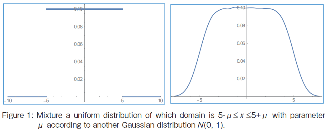
Consider a probability variable of a uniform distribution x (5-μ≤ x ≤ 5+μ), μ=0．Then the resultant shape is staircase shaped in the left one of Figure 1. Then suppose that the parameter μ to be distributed according to the standard normal distribution N (0, 1). The result is illustrated as shown in the right one of Figure 1. The distributions in the example are not conjugate.

【192 頁】

�A Normal Distribution with a Parameterized Mean

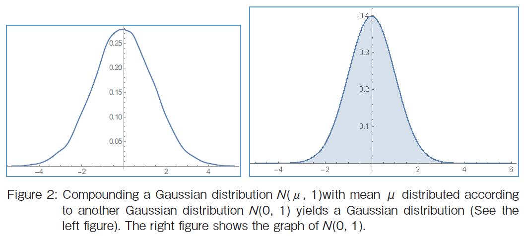
The second example shows conjugate distributions. The Gaussian family is conjugate to itself with respect to a Gaussian likelihood function. If the likelihood function is Gaussian, choosing a Gaussian prior N (0, 1) over the mean will ensure that the posterior distribution is also Gaussian as shown in Figure 2. The distributions in the example are conjugate.

4　Conjugate Distributions in Latent Dirichlet Allocation Model

In the section, I shall explain the LDA model and show the visualization of the conjugate distributions. The LDA (Latent Dirichlet Allocation) model is a widely-used multi-topic document model based on Baysian intefrence method. Although the original LDA algorithm details are described in [1], we shall explain the frame simply. The LDA model is often used for topic extractoin. In the LDA model, each topic is supposed to have a set of relted words. For example, suppose that there are two topics 【193 頁】 “economics” and “disaster”. Each topic has probabilities of generating various words. For example, suppose that the topic “economics” has a related word set {“exchange”, “finance”, “stock”, “yield” } and the word distribution for the topic “economics” is supposed to be (0.3, 0.2, 0.4, 0.1). Suppose that the word generating distribution is a multinominal distribution. If the input sentense is “stock finance yield stock exchange stock”, the probability of the sentence becomes ×0.3×0.2×0.4³×0.1. One document is supposed to have several topics. The topic distribution for the document may be (0.7, 0.3) (in the case of an economic related document) or (0.2, 0.8) (in the case of a disaster related document). To express the possible various distributions, we use Dirichlet distribution by using a hyper parameter α． On the same way, we define per-topic word distribution by Dirichlet distribution by using another hyper parameter β.
　In Bayesian probability theory, if the posterior distributions p (θ| x ) are in the same family as the prior probability distribution p (θ), the prior and posterior are then called conjugate distributions, and the prior is called a conjugate prior for the likelihood function. In the Latent Dirichlet Allocation model, the likelihood function is Multinomial and the prior function is Dirichlet. There the Dirichlet distribution is a conjugate prior and then the posterior function becomes also Dirichlet. The posterior function is a parameter mixture distribution where the parameter of the likelihood function is distributed according to the given Dirichlet function.
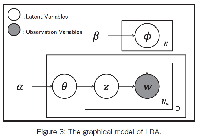
　We will explain the LDA method. There the used symbols are as follows:

α is the parameter of the Dirichlet prior on the per-document topic distributions,
β is the parameter of the Dirichlet prior on the per-topic word distribution,
θ_i  is the topic distribution for document i,
φ_k is the word distribution for topic k,
z_ij  is the topic for the j th word in document i, and
w_ij  is the specific word.

【194 頁】

The w_ij  are the only observable variables, and the other variables are latent variables. The graphical model is illustrated in Figure 3. φ is a Markov matrix of which size is K × V (V  is the dimension of the vocabulary) each row of which denotes the word distribution of a topic. The LDA generative process for a corpus D consisting of M documents each of length N_i  is as follows where K denotes the number of topics:

1. Choose θ_i 〜 Dir(α), where i ∈{1, ..., M } and Dir(α) is the Dirichlet distribution for parameter α

2. Choose φ_k 〜 Dir(β), where k ∈{1, ..., K }

3. For each of the word positions i, j, where j ∈{1, ..., N_i }, and i ∈{1, ..., M }
(a) Choose a topic z_ij 〜 Multinominal(θ_i ).
(b) Choose a word w_ij 〜 Multinominal(φ_zij ).

We want to obtain an estimate of Z that gives high probability to the words that appear in the corpus. z_ij represents the topic for the j th word in document i. This problems becomes a maximum a posteriori estimation of P (W, Z, Θ, Φ |α, β). By an integration concerning θ and φ (i.e., marginalization), the expression becomes a simple one, P (W, Z |α, β). Therefore, we want to obtain Z so that P (Z | W, α, β) is maximum. The W is given data. The cost of the calculation is too high because the estimation space size is the number of topics (K ) to the power of the dimension of the vocabulary (V ), K^V. Namely each word has K options independently. So instead of that, a random walk search method by Gibbs sampling is widely used.
　In the LDA model, the likelihood function is Multinomial and the prior distribution is Dirichlet. The normalized product of these two components yields also Dirichlet distribution. The Multinomial and Dirichlet distributions are conjugate distributions.

(1)Visualization of Dirichlet distribution for β=(2, 2)
　Suppose that concerning the topic “sports”, there exist two words “game” and “efforts”. We want to make the model of the word distribution about the topic “sports” by using Dirichlet distribution. The hyper-parameter of the Dirichlet distribution is supposed to be β=(2, 2). Then the resultant one-dimensional Dirichlet distribution is illustrated as shown in Figure 4 where p₁ and p₂ represent each word appearance probabilities. The horizontal axis in Figure 4 is p₁. The variable p₂ can be calculated as p₂ =1 - p₁. The vertical axis shows the probability density function.

【195 頁】

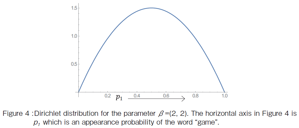
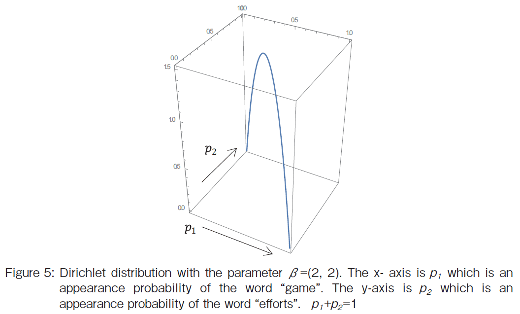
The Dirichlet distributions in Figure 4 and 5 is the same Dirichlet distribution. However, the Dirichlet distribution illustrated in a three-dimensional space is defined only on the line p₂ = 1 - p₁ on the p₁ and p₂ plane.

(2)Visualization of Multinomial distribution with a fixed parameter

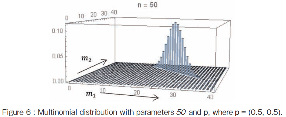
Next I shall make a distribution model for the number of times outcome number i  is observed over the 50 trials where each trial results in exactly one of two possible outcomes(“game” or “efforts”), with probabilities (Pgame, Pefforts)=(0.5, 0.5). Then if the random variables m_i  indicate the number of times outcome number i is observed over the 50 trials, the vector M = (m₁, m₂ ) (Σm_i =50) follows a 【196 頁】 Multinomial distribution with parameters 50 and p, where p = (0.5, 0.5). Figure 6 shows the Multinomial distribution. The x-axis is the m₁ times and the y-axis is the m₂ times. The vertical axis (or z-axis) is the probability distribution. The point with the highest probability is M = (25, 25).

(3)Visualization of Multinomial distribution with a parameter over a Dirichlet distribution (A)
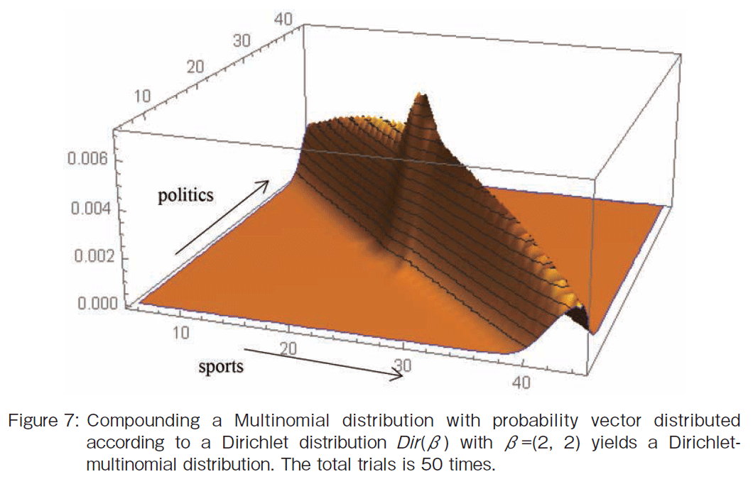
　Although the parameter of Multinomial is fixed in Figure 6, let the parameter be distributed according to Dirichlet Dir(β) with the parameter β=(2, 2). The compound probability distribution is shown in Figure 7. The Multinomial distribution has no width. However, the distribution has width as shown in Figure 7. The point with the highest probability is still at M =(25, 25).

【197 頁】

(4)Visualization of Multinomial distribution with a parameter over a Dirichlet distribution (B)
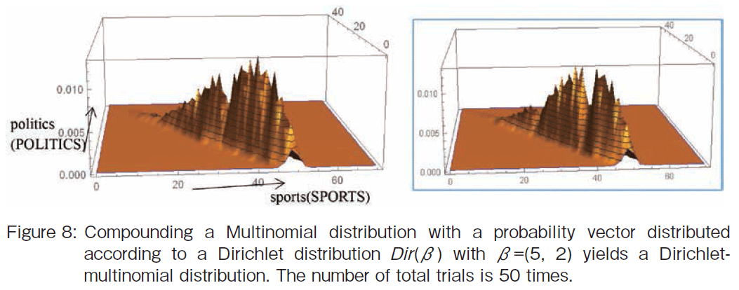
　Next I shall make a distribution model for the number of times outcome number i  is observed over the 50 trials with a probability vector distributed according to a Dirichlet distribution Dir(β) with β=(5, 2) (See Figure 8). The words are “game” and “efforts”. This shows compound a Multinomial distribution with a probability vector distributed according to a Dirichlet distribution yields again a Dirichlet-multinomial distribution. As shown in Figure 8, the point with the highest probability is shifted from the point (25, 25) so that the times for “game” is greater than the times for “efforts”. The shape of the histogram looks saw-toothed because this is a result of an at random simulation. The shapes change with each simulation. Figure 8 shows two simulation results.

(5)Visualization of compound probability distributions in LDA model
　In the LDA model, z_ij  that is the topic for the jth word in document i  is generated by using the Multinomial distribution Multinominal(θ_i ) where θ_i  is the topic distribution for document i . Let us consider a concrete example.
　Suppose that there are two topics which are “SPORTS” and “POLITICS” and that the number of words in document i  is 50. Choose θ_i 〜 Dir(α), where Dir(α) is the Dirichlet distribution for parameter α=(5, 2). The resultant topic distribution is the same one as one in Figure 8 of the previous visualization (4). The topic distribution corresponds to z_ij .
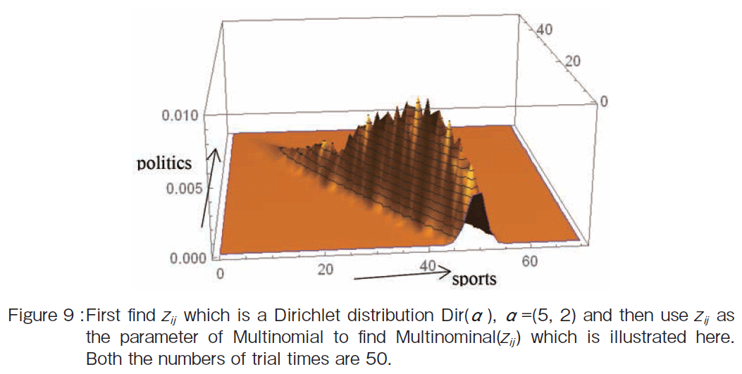
　Next consider φ_zij  which is the word distribution for topic z_ij . Suppose that there are two words which are “sports” and “politics”. The word “sports” is supposed to appear only under the topic “SPORTS”. In the same way, the word “politics” is supposed to appear only under the topic “POLITICS”. Then z_ij  which is the topic for the j th word in document i is the same as φ_zij  which is the word distribution for topic z_ij .
　Then the word distribution w_ij  follows Multinominal(φ_zij ) (See Figure 9) where the number of trial time is 50. The x-axis is an apperance time of word “sports” and the y-axis is an appearnce time of word “politics”.
　In this simulation we suppose that z_ij  is the same as φ_zij  in order to make the calculation process simple. By using z_ij  which is a Dirichlet distribution as the parameter of Multinomial, Multinominal(z_ij ) is calculated. The results also becomes a Dirichlet distribution as shown in Figue 9.

【198 頁】

5　Conclusion

The paper shows the visualization of conjugate distributions appeared in the LDA model. The LDA model is widely used for topic extraction. There the likelihood function is Multinomial and the conjugate prior is Dirichelt distribution. As a result, the posterior distribution becomes also Dirichlet, precisely Dirichlet-Multinomial distribution. The constraint of the visualization is that we can use just only three-dimensional space. Hence, the number of topics must be two. Compared with the number in a practical use, the number two is too small. However, the visualization is so helpful so that we can understand the conjugate distributions. Because compound probability distribution is a complicated idea, the visualization as shown here would help many students have the clear images of them.
　This is our first step visualization concerning the Bayesian inference. As the future works, we would like to continuously visualize Gibbs sampling so that we can illustrate the effects by the conjugacy.

References

[1] Blei, D.M., A.Y. Ng, and M.I. Jordan, Latent dirichlet allocation. Journal of Machine Learning Research, 2003. 3: p. 993-1022.

[2] Griffiths, T.L. and M. Steyvers, Finding scientific topics. Proceedings of the National Academy of Sciences, 2004. 101 (Suppl. 1): p. 5228-5235.

[3] Fink, D., A Compendium of Conjugate Priors. 1997.

[4] Raiffa, H. and R. Schlaifer, Applied Statistical Decision Theory. Division of Research, Graduate School of Business Administration, 1961.

[5] Bishop, C.M., Pattern Recognition and Machine Learning 2006: Springer.
(His materials are avaiable on http://research.microsoft.com/en-us/um/people/cmbishop/)

[6] Chib, S., Bayes regression with autoregressive errors. Journal of Econometrics, 1993. 58: p. 275-294.

【199 頁】

[7] Li, A.Q., et al., “Reducing the sampling complexity of topic models,” in Proceedings of the 20th ACM SIGKDD international conference on Knowledge discovery and data mining2014, ACM: New York, New York, USA. p. pp. 891-900.

[8] Darling, W.M., “A Theoretical and Practical Implementation Tutorial on Topic Modeling and Gibbs Sampling.”, 2011, http://u.cs.biu.ac.il/~89-680/darling-lda.pdf

[9] Carpenter, B., “Integrating Out Multinomial Parameters in Latent Dirichlet Allocation and Naive Bayes for Collapsed Gibbs Sampling,”, 2010, http://lingpipe.files.wordpress.com/2010/07/lda3.pdf