【1 頁】

Visual Explanation of Deformation Theories in Shape Analysis

Yukari Shirota¹⁾，Takako Hashimoto^2）

ABSTRACT

In the paper we explain the deformation theories in shape analysis. The Geometry Driven Statistics offers a new horizon of the statistical methods. Using a thin-plate interpolation, the given configuration with landmark coordinates is featured by the principal warps which are eigenvectors of the bending energy matrix. In addition, the deformation between two configurations can be described by an affine transformation component and a non-affine transformation. The non-affine transformation can be described by partial warps. Seeing the partial warps help a lot us to understand the features of the deformation. We apply the deformation theories to a tiny economics deformation analysis. The concrete example will be helpful so that economics students can understand the deformation theories. In addition, the way of applying the shape analysis method is explained through the concrete example.

1 Introduction

The paper explains deformation theories in shape analysis. We can see various formations in our world. For example, they are formations made by American football players, and formations made by flying aircrafts. In the data analysis, we use many relationship diagrams. For example, the diagrams visualize a relationship among group companies or among economic entities. There, the small distance means a tight connection between two entities.
　The formation may be changed to another formation when time goes by. We call the formation change a deformation. For a long time, it has been of great importance to measure shapes of objects in morphology. In the shape analysis, it is important how to compare different shapes; they have different sizes and orientations. The process of transforming different sets of data into one coordinate system is called image registration using register marks. That is a tough problem and the image registration problem had been discussed for a long time. However, the research results conducted by University of Leeds members and others made remarkable progresses in shape analysis to solve the problem[2]. The research field is called “statistical shape analysis” or “geometry driven statistics” [3, 4]. The field of 【2 頁】 statistical shape analysis involves methods for the study of the shapes of objects where location, rotation and scale information can be removed to compare the shapes [1].
　The recent outputs by the Mardia who is the main researcher of the field include various fields such as “Bayesian methods in structural bioinformatics,” “statistical approaches to three key challenges in protein structural bioinformatics,” and “Alcohol, babies and the death penalty: Saving lives by analysing the shape of the brain” [5-8]. In [7], Mardia, Bookstein, and Kent describe changes of shape in the brain and how to analyse the brain shapes statistically, and how to distinguish affected brains from normal ones. They revealed evidence of damage to the brain by the statistical methods. To compare the two shapes, we use landmarks which illustrate the corresponding pairs. The landmarks are translated, rotated, and scaled so that they are lined up and matched as closely as possible. The procedure is known as a generalized Procrustes analysis [7].
　The shape analysis applications include medical imaging and morphometrics for biology. Mardia describes that non-Euclidean data driven mainly by underlying geometry arise in a variety of important new applications generated by areas such as bioinformatics, meteorology, new energy sources, and finance. In these applications, variables are observed on several different manifolds: circle, sphere, cylinder, space of orthogonal matrices, Stiefel manifold, Grassmann manifold, shape spaces[5]. In addition, some statistical challenges by the statistical shape analysis were conducted in managing the big data [9]. Although there are many papers on biology and medical imaging fields, as far as we know, there are no economics analysis paper by this statistical shape analysis. We would like to apply the statistical shape analysis methods for the economics analysis. The problem is that how to project the higher attribute space which we would like to analyse to the geometry world. In other words, we would like to find the geometry/formation in the economics applications so we can analyse them using the shape analysis methods.
　The purpose of the paper is to explain the math processes concerning the thin-plate spline interpolation and the partial warp components which are the core theorems for the shape analysis. We shall explain them visually so that the readers can easily understand the math processes. Another purpose of the paper is to challenge of applying the shape analysis method to the economics analysis using a concrete example. Suppose that there are five companies in a company group and define the trading quantity indices among them. The time-change on the relationships can be illustrated in the partial warps.
　In the next section, we shall explain the target problem which is the time-change analysis of the company relationship. In Section 3, we shall analyse the change using the thin-plate generation or so. Then the acceleration of changes can be expressed by the principal components called the partial warp. Finally we shall conclude the paper, considering points for using shape statistical methods in the economical applications.

2 Mathematics for Deformations

In the section, we shall explain the thin-plate spline interpolation, eigenvectors of its bending energy matrix and partial warps, which are cited from [3, 4, 8]. In this paper, we skip the Procrustes distance in order to focus on the partial warps.

【3 頁】

We concentrate on the m = 2 dimensional case. In other words, we shall analyse two dimensional data such as diagrams, not three dimensional data.
　Suppose that there are k landmarks in R², t_j , j = 1, ..., k, on the first figure mapped exactly into y_j , j = 1, ..., k, on the second figure, namely there are 2k interpolation constraints,

and we write Φ(t) = (Φ₁(t), Φ₂(t))^T,　j = 1, ... , k, for the two dimensional deformation. Let

so that T and Y are both (k×2) matrices. A pair of thin-plate splines is given by the bivariate function

where, Φ is (2×2), t is (2×1), c is (2×1), A is (2×2), W^T is (2×k), s (t) = (σ (t-t₁), ..., σ (t-t_k))^T is (k×2), and

If ||h|| = 0, then σ (h) = 0. Matrix A means the affine transformation part and the matrix W is corresponding to the non-affine transformation part. From the given T and Y data, we can find the unknown A and W.
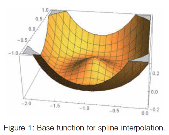
　Figure 1 illustrates the σ(t-t_i) function where t = [x, y ]^T, t_i = [-1, 0]^T. The function has one local maximum point at the given t_i . The deformation from T to Y can be interpolated by the k base functions σ (t-t_i) = ||t-t_i||² log (||t-t_i||), i = 1, ..., k.

Additional constraints in order for the bending energy below to be defined as follows:

1_k is the k-vector of ones. The pair of thin-plate splines which satisfy the above constraints are called natural thin-plate splines, represented by W. The expression can be re-written in a matrix form

【4 頁】

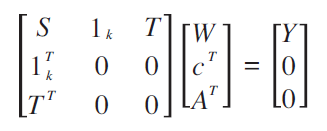
where (S )_ij = σ (t_i -t_j ) is (k×k). The matrix

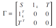
is (k+3, k+3), symmetric positive definite and so the inverse exists, provided the inverse of S exists. Hence,

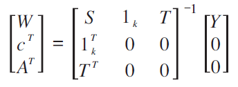
So we can obtain the concrete expression the affine transformation matrix A and the spline matrix W. The bending energy matrix is defined as Г¹¹ in the following expression.

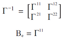
We call Г¹¹ the bending energy matrix B_e of which size is (k×k). It can be proved that the transformation of Φ(t) = (Φ₁(t), Φ₂ (t))^T = c + At + W ^T s (t) minimizes the total bending energy of all possible interpolation functions mapping from T to Y.
　After an eigen-decomposition of B_e we can get (k-3) non-zero eigenvalues λ₁, λ₂, ..., λ_k-3 with (k-3) corresponding eigenvectors γ₁, γ₂, ... ,γ_k-3. We call the eigenvectors principal warp eigenvectors. Because (S )_ij = σ (t_i -t_j ) has no Y related data and then Г has no Y related data, in B_e there is no information of Y. In other words, the principal warp eigenvector expresses the principal component of the formation T. We define (k-3) principal warps P_j (t) as follows:

where γ_j^T is (1×k), s(t) = (σ(t-t₁), ..., σ(t-t_k))^T is (k×2), and P_j (t) is (1×2). Given the x and y coordinate, a value is calculated which expresses the principal warp of the point.
　Next, we would like to express the deformation T to Y, using the principal warps of T. In other words, we shall express the deformation from the standpoint based on the T formation. We call the deformation partial warps and define as follows:

where Y^T is (2×k), γ_j is (k×1), γ_j^T is (1×k), s(t) = (σ(t-t₁), ... σ(t-t_k))^T is (k×2), and R_j(t) is (2×2).
　The partial warp is a bivariate function of which size is (1×2). The warp part W^Ts (t ) can be expressed by the addition of (k-3) partial warps. The math process may be difficult to understand. However, the following sections offer the concrete example visually, which will be useful for the understanding.

【5 頁】

3 Trading Quantity Relationship

In the section, we shall define the target economics problem.
　Suppose that five automobile companies and that we know the trading quantities and investment amounts among them so that we can define the trading amount index trakingQ_ij between two companies. If they are countries, not companies, the import and export amounts would be used to define the index. From the index, we can define the distance between two companies. For example, distance r_ij may be define as where k is positive constant value. When {tradingQ_ij } are given between any two companies, we can define the individual distance between the two companies and we can set the simultaneous equations. In general we cannot solve the equations in two dimensional world. Then higher dimensional world is required to express the solution. However, we would like to make the two dimensional formation data for the visualization. Then some process to reduce the number of dimensions is needed.
　In the following we shall suppose that two dimensional formation T₀ and Y₀ are given. This is because we would like to visualize the deformation in 2 dimensional world. The given form data T₀ and Y₀ are shown in Figure 2. The figure data are artificially defined by us and there is no relationship to the real company data.

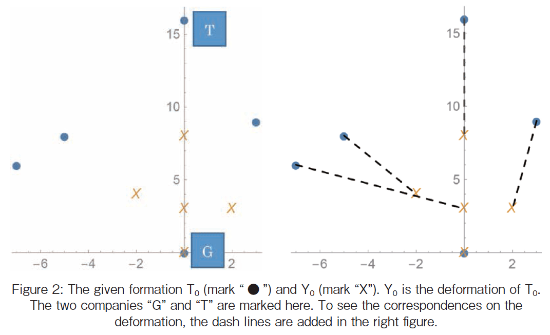
We made the sample data so the deformation would mean that company T and G increases the trading and that the other three companies increase the trading with G.

【6 頁】

4 Visualization of Trading Quantity Relationship

In the section, we visualize the deformation process using the sample data given in Section 3.
　First the two figures are transformed to the pre-shape. The term pre-shape means that is centered to the point (0, 0) and scaled by the centroid size but that is not yet rotated [3]. Figure 3 shows the preshapes named T and Y.

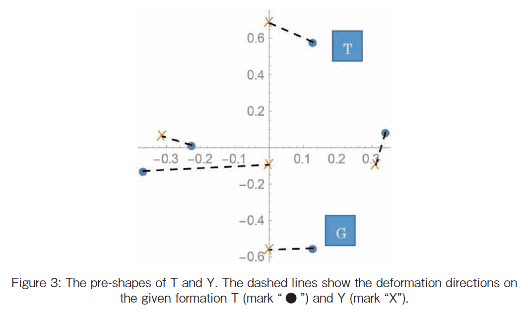
The deformation is divided to the two parts; they are the affine component and the non-affine component. We call the non-affine component the partial warps. In the section 2, we explain the deformation

In the expression, At means the affine component and the W^T s (t) is the partial warp. In the partial warp component, s(t) means the linear combination of five base functions for spline interpolation with the local maximum at the given landmarks of the T (See Figure 1); the number of landmarks is five. The matrix W ^T means the coefficients of the spline base functions. The non-affine component is also divided to the partial warps. In the case, k=5 landmarks and m=2 dimension. Then the number of the principal components is k-(m+1)=2. Then the number of partial warps is also two.
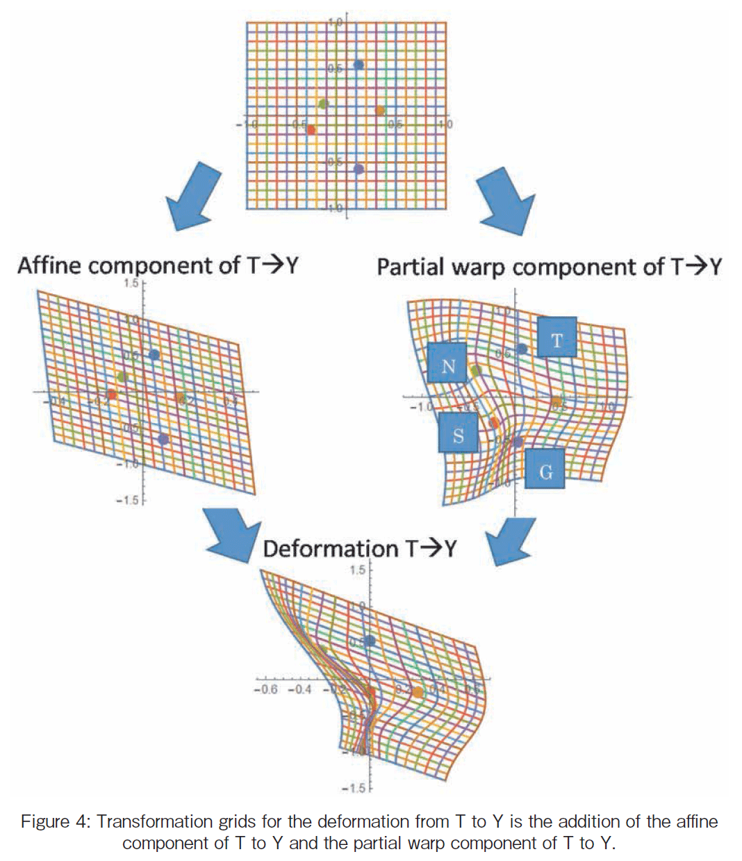
　We shall illustrate the Cartesian transformation grids, using a pair of thin-plate splines for the deformation form T to Y. Figure 4 shows the transformation grids for the deformation from T to Y. The top grid shows the initial square grid placed on the pre-shape T. In Figure 4, the bottom figure shows the 【7 頁】 pre-shape Y. The corresponding grid lines are skewed and warped by the deformation. Roughly speaking, we can see that some warps are found around the company “T” and “G” line; the data are artificially made and there is no relationship to the real ones. The company “S” gets nearer to the “T” and “G” line. On the other hand, company “N” a little bit gets away from the “T” and “G” line. To express the warps, the orthogonal grid lines are tortured.

【8 頁】

Next we shall illustrate the non-affine transformation component. For the case, the bending energy matrix is as follows:

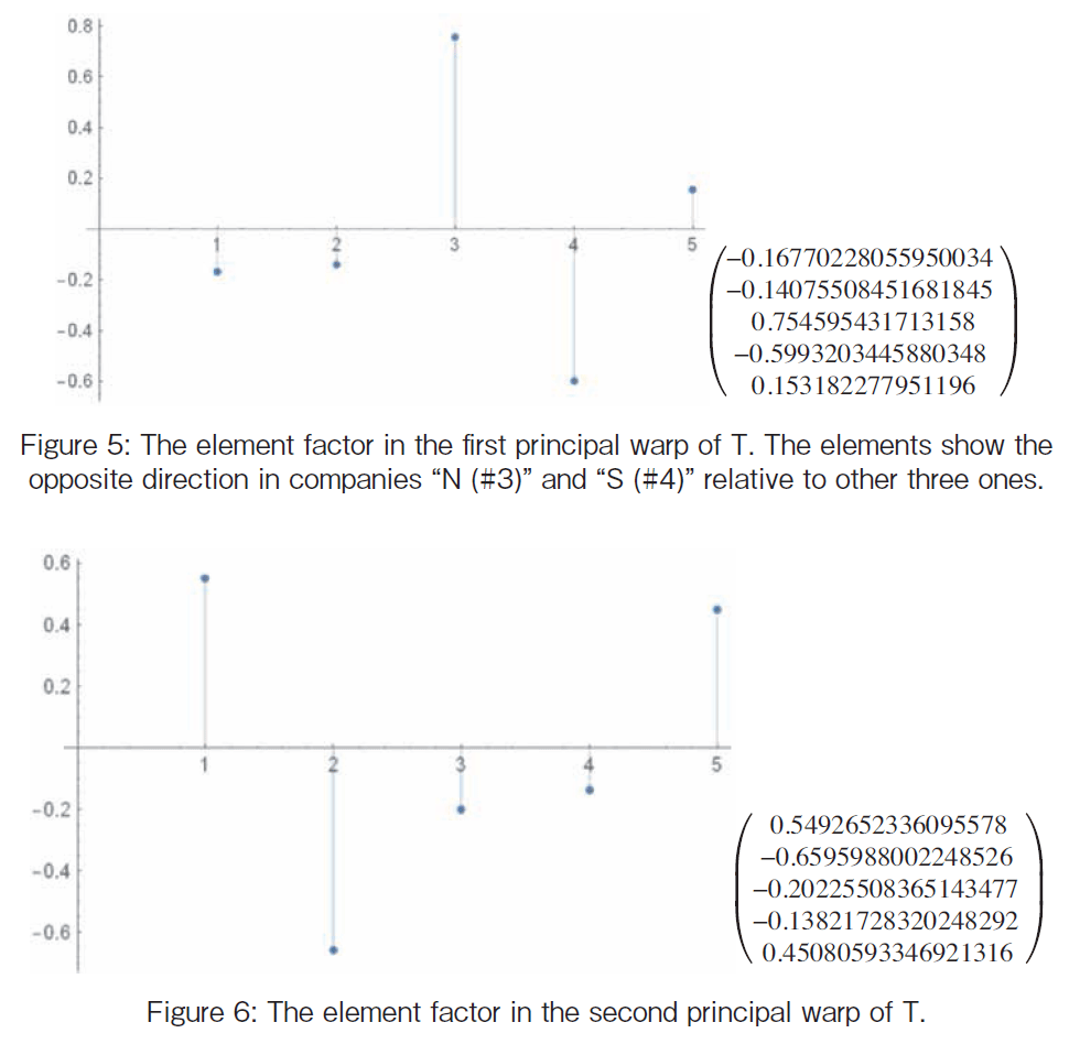
We calculate the eigenvectors and eigenvalues of the matrix. Then, we shall find the principal warp P_j(t) = γ_j^T s(t), j = 1, 2. The T formation is represented by the two eigenvectors of the bending energy matrix as shown in Figure 5 and 6. The eigenvalues are 7.9 and 3.0 which shows that the first principal warp has a larger effect than one of the second principal warp. The two principal warps P_j(t) = γ_j^T s(t) are found as follows:
　The first principal warp function is

【9 頁】

The second principal warp function is

We shall illustrate the principal warps of the T formation as surfaces in Figure 7.

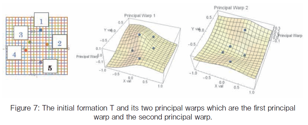
The principal warps has no information of Y. The principal warps express the relationship among the five landmarks on T; the significant part is (S )_ij = σ (t_i -t_j ) of which size is (k×k). Just seeing the initial T formation, we can see that the nearest pair is # 3 and # 4. The first principal warp expresses the nearest pair by making # 3 up and # 4 down on the thin-plate. In the second principal warp, the movement that companies # 3, # 4, and # 5 get near to the vicinity of the “T(# 1)-G(# 5)” line. Especially # 2 landmark gets near the T-G line. The movement is made getting # 1 and # 5 up and getting # 2 down.
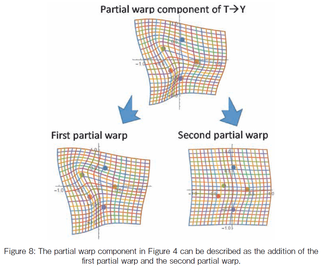
　The geometry driven statistics offers a new interpretation of the relationship diagram by the natural thin-plate interpolation. The resultant transformation grids give us how the thin-plate has been bent. The eigenvectors, the principal warps, can tell us the principal component of the non-affine formation. In the non-affine deformation from T to Y, the formation Y also has its eigenvectors. The difference between the eigenvectors of T and eigenvectors of Y can be described based on the eigenvectors of T, which is the partial warps R_j(t) = Y^T λ_j γ_j γ_j^T s(t).
　The non-affine formation component of the deformation is called a partial warp component and can be described as an addition of each partial warps. In the example, because the number of the landmarks is five, we can obtain the first and second partial warps (See Figure 8).

【10 頁】

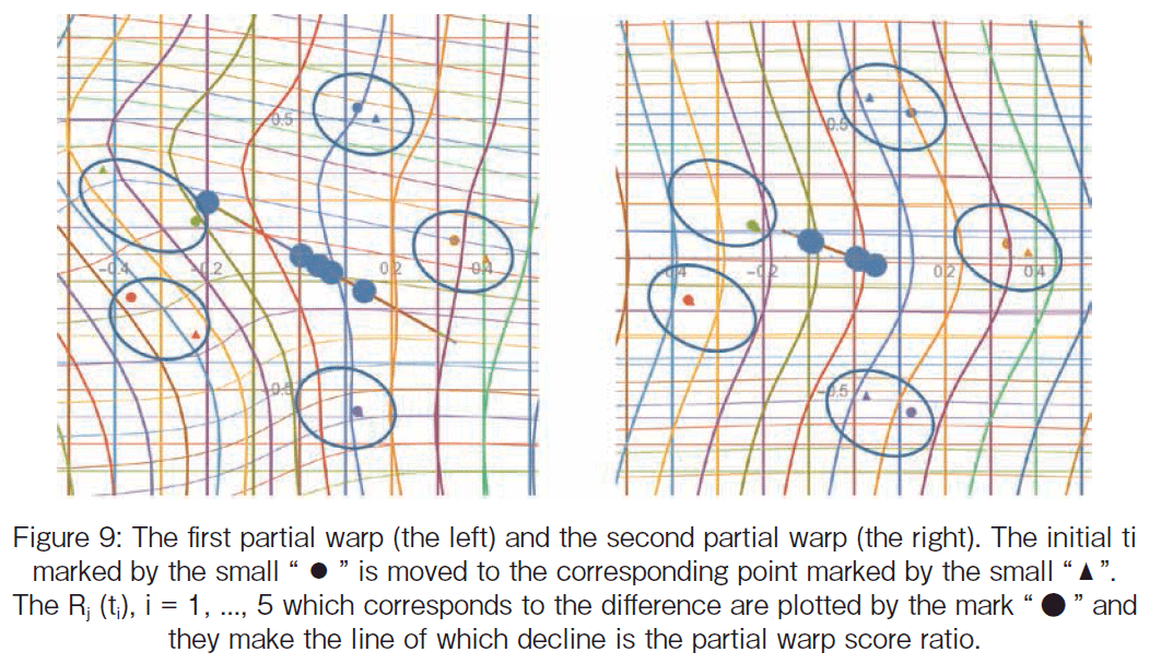
The partial warps in Figure 8 show T + R_j (t) transformation. Only R_j (t) is illustrated in Figure 9. Input the five landmark t of T, we calculate the vector R_j (t) of which size is (2×1) and plot them. Let us see the first partial warp in Figure 9. The landmarks # 1 and # 5 hardly move and other three move. Only # 2 moves away from the T-G line and # 2 and # 3 get near to the T-G line. The coordinate difference on each landmark R₁(t) is plotted on the line. The second partial warp in the right figure shows that the T-G line moves to the right direction. The coordinate difference on each landmark R₂(t) is plotted on the line as well as R₁(t). The circle mark “ ● ” on the line represents the contribution of each landmark t_i onto the partial warp. If t_i has no movement by the partial warp, then the difference is zero and the mark “ ● ” is plotted at (0, 0). The decline of the line can be calculated as a ratio of Y^T λ_j γ_j which is (2×1); The Y^T γ_j is called the j -th partial warp scores for Y from T. Figure 9 shows that both decline coefficients are negative and that the first partial warp decline is larger than the second one.

【11 頁】

5 Conclusion

In the paper, we describe an application of geometry driven statistics to the economics example. When a set of landmarks coordinates is given, the shape analysis method can give us the principal warps of the configuration as eigenvectors of the bending energy matrix. The shape analysis method can be applied to various economics analyses. In the paper, we suppose that the relationship diagram among automobile companies is given. The company relationship diagram is not easy to be obtained as two dimension diagram; some dimension reducing process is required for that. However, we have many two dimensional plot data in the field of economics. They include various kinds of big data. As future work, we will analyze the data by the shape analysis. In addition, the deformation between two formations can be expressed by the partial warps. The partial warp can be expressed by the eigenvector and the impact factor of each partial warp can be expressed by the eigenvalue. We have been using the eigenvectors through Principal Component Analysis, Singular Value Decomposition and so forth. The resultant eigenvectors are significant to understand the data relationship or correlation. Then visualization of the eigenvectors helps us understand that easily. We will continue to apply the shape analysis methods to many economics data analysis.

References

[1]   Dryden, I.L. and K.V. Mardia, Statistical shape analysis with Applications in R (Second Edition). 2016: J. Wiley Chichester.

［2］  Kanti, M. Geometry-Driven Statistics and its Cutting Edge Applications: Celebrating Four Decades of Leeds Workshops. in The 33rd Leeds Annual Statistical Research Workshop. 2015. Mardia Kanti et al.: Department of Statistics, University of Leeds.

【12 頁】

［3］  Dryden, I.L. and K.V. Mardia, Statistical shape analysis. Vol. 4. 1998: J. Wiley Chichester.

［4］  Dryden, I.L. and J.T. Kent, Geometry Driven Statistics. 2015: Wiley Online Library.

［5］  Kanti, M. Some Aspects of Geometry Driven Statistical Models. in Leeds Annual Statistical Research Workshop: Statistical Models and Methods for non-Euclidean Data with Current Scientific Applications. 2013. Department of Statistics, University of Leeds.

［6］  Bayesian methods in structural bioinformatics. 2012: Springer Science & Business Media.

［7］  Mardia, K., F. Bookstein, and J. Kent, Alcohol, babies and the death penalty: Saving lives by analysing the shape of the brain. Significance, 2013. 10(3): p. 12-16.

［8］  Mardia, K.V., Statistical approaches to three key challenges in protein structural bioinformatics. Journal of the Royal Statistical Society: Series C (Applied Statistics), 2013. 62(3): p. 487-514.

［9］  Laha, A.K. Big Data Analytics in Management: Some Statistical Challenges and Opportunities. in The 33rd Leeds Annual Statistical Research Workshop. Department of Statistics, University of Leeds.