Analysis of Indian Automakers’ Resilience after COVID-19
—Comparison between Indian and Japanese Automakers—
Basabi Chakraborty (Iwate Prefectural University, Madanapalle Institute of Technology and Science)
Bonthala Sreekanth (Madanapalle Institute of Technology and Science)
Yukari Shirota (Gakushuin University)
The present paper analyzes the Market Capitalization (MC) growth rates of Indian automakers, highlighting their impressive recovery from COVID-19. To assess this growth, the study compares Indian automakers to their Japanese counterparts using AI-based clustering methods, focusing on Amplitude-based clustering to evaluate growth variance. The study avoids data standardization to preserve variance data. After the amplitude-based clustering, dimensionality reduction techniques, including PCA, t-SNE, and UMAP, are applied to the distance matrix obtained from clustering. The results consistently show that Indian automakers have significantly higher recovery and growth rates than Japanese automakers.
In this paper, the Market Capitalization growth rates of Indian automakers are analyzed. The Indian automakers have shown splendid growth and here we would like to explore the cause of high-speed recovery of Indian automakers from COVID-19. To evaluate the Indian automakers’ highest growth level, we will conduct a comparison to that of Japanese automakers. The data used is Market Capitalization (hereafter MC) instead of stock prices, because MC data movement may be continuous as MC = [stock price] x [the number of issued stocks]. The method used is the AI-based clustering method. As we would like to evaluate growth variance/amplitude, for example, which company has the highest growth rate, Amplitude-based clustering is used. The clustering method with the data standardization cannot be used, because the data standardization removes the large variance of the data. The distance matrix among the companies can be obtained from the Amplitude-based clustering. In our analysis, the dimensional reduction for the distance matrix is conducted, so that the appropriate axis can be obtained such as the first PCA axis etc. In the analysis, three different dimensional reduction methods, PCA, t-SNE, and UMAP are used. As a result, the three kinds of results showed that the Indian automakers had much higher recovery/ growth rates compared with the Japanese automakers.
In the next section, the data details are explained. Then our previous work with the HRP clustering method is described. In Section 4, the Amplitude-based clustering and dimensionality reduction with 【184頁】 resultant distance matrix has been described. In Section 5, the results are discussed. Finally, Section 6 concludes the paper.
In this section, the data used in the analysis are described. The objective of this analysis is to estimate the automakers’ resilience after the decline by COVID-19. Then, the data period is set from March 31st, 2020 to March 31st, 2024. We have analyzed the four-year movement of MC. The quarterly data is used from the database Web Orbis of Bureau van Dijk (BvD). To evaluate the Indian automakers’ stock movement, we thought that a comparison is needed and representative Japanese automakers’ data are added. As the data, 28 automakers with the largest net sales amounts at the end of March 2024, are selected. The total number of automakers is 28 of which six are Indian companies and 22 Japanese companies are included.
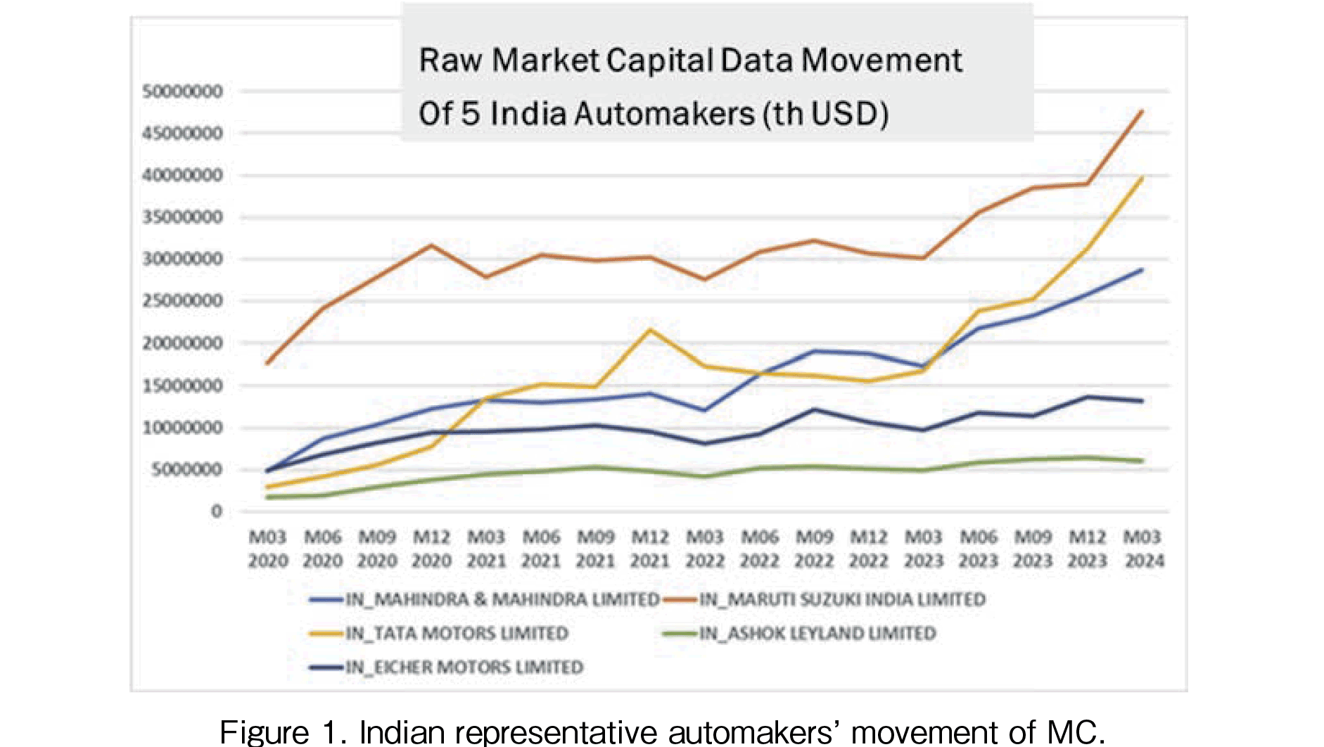
In Figure 1, the Indian representative automaker’s MC movement is presented. The largest MC company is Maruti Suzuki. The second largest company is Tata and the third is Mahindra & Mahindra. After COVID-19, these Indian automakers have been rapidly growing. The foundation of the modernization of the Indian automobile industry was laid in 1981 with the establishment of the Suzuki joint venture. The history of Maruti Suzuki is as follows: in 1981, it was a local government-owned company; in 1982, Suzuki invested in it and it became a semi-private joint venture; in 2006, the Indian government sold its entire stake in it and it became a fully privatized private joint venture; in 2007, the company name was changed to Maruti Suzuki India. In the global automotive market, Toyota, VW, and 【185頁】 others are the top players, but in India, Maruti Suzuki is the top player, followed by Tata Motors and Mahindra & Mahindra, and then Hyundai Motor Company of Korea. This is because small cars are heavily favored in terms of taxation and users are very price-sensitive. As a result, Suzuki, Hyundai, and local automakers that have been vigorously developing models that meet Indian needs have a high presence in the market. The market is also very competitive in terms of price.
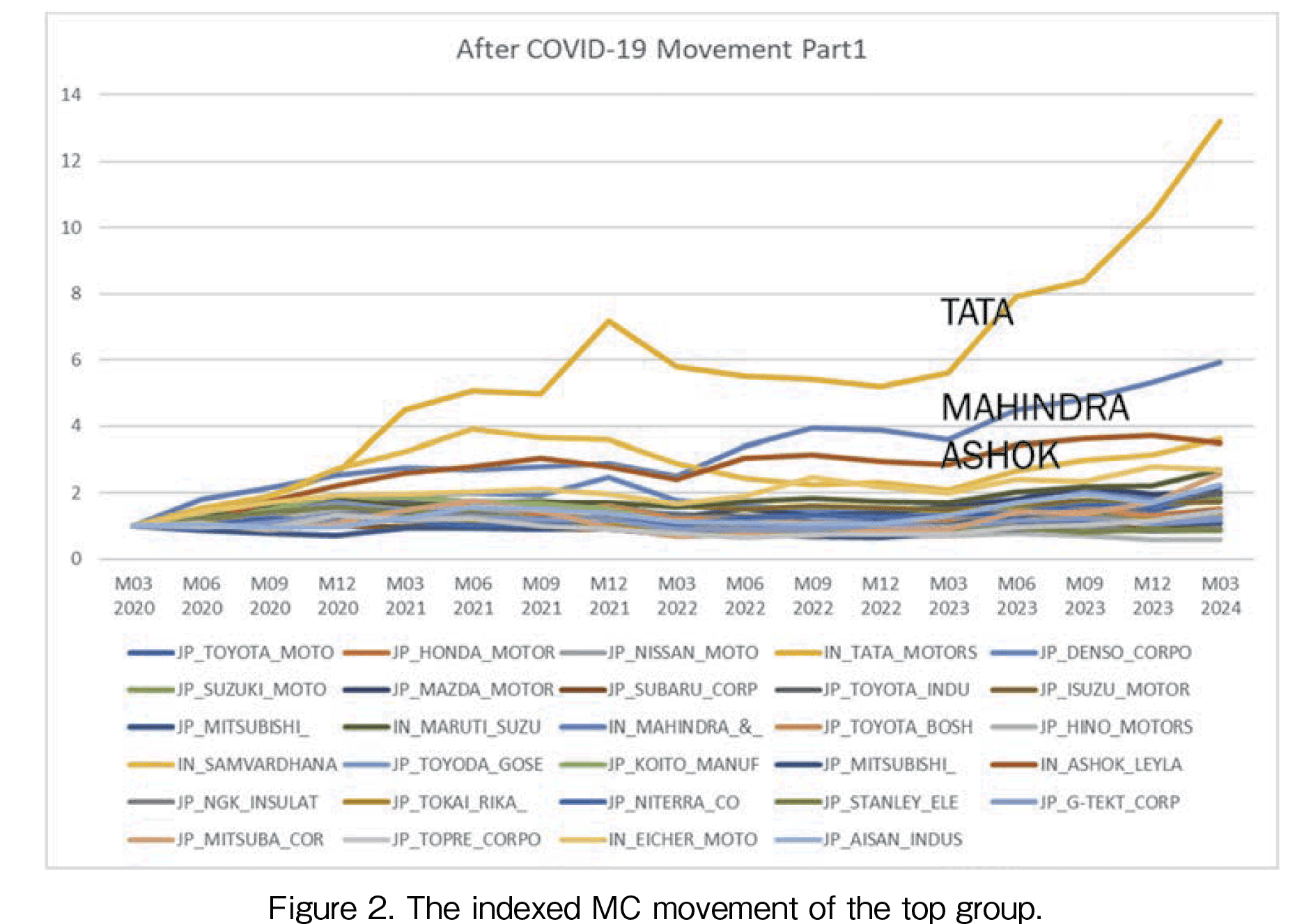
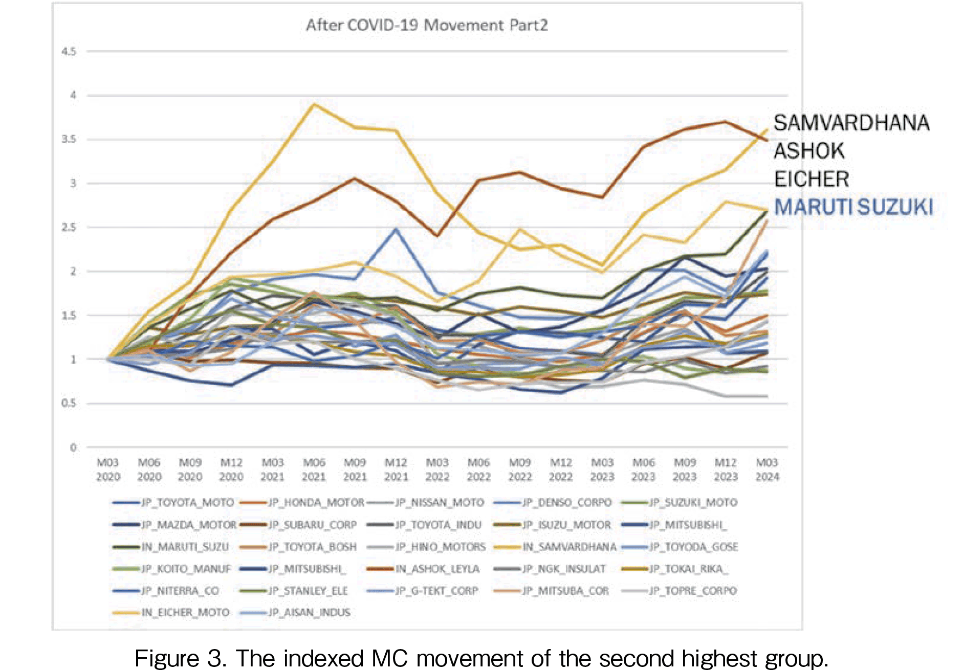
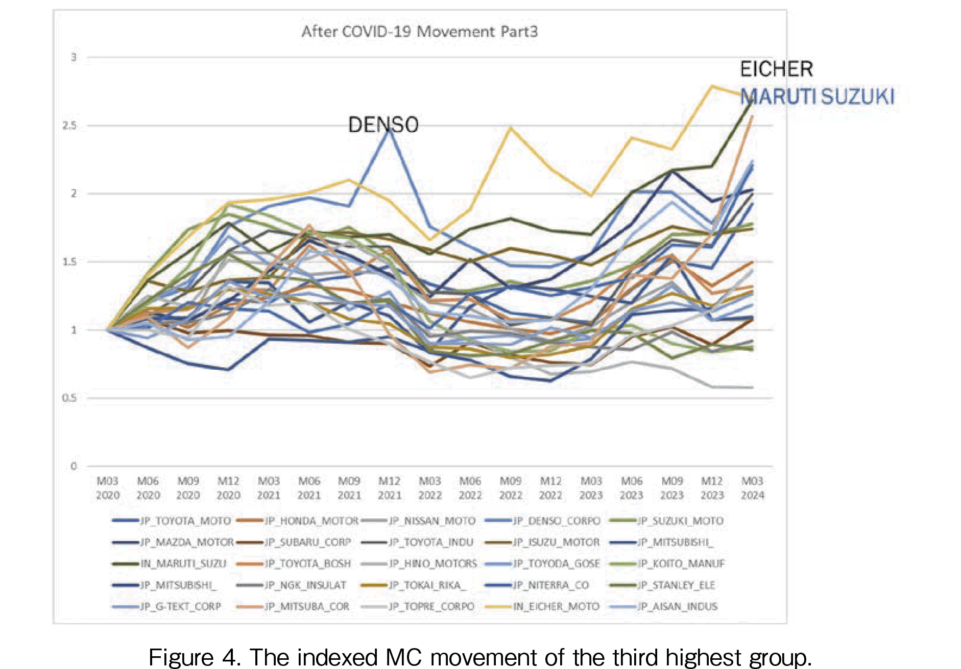
In Figures 2 to 4, the indexed MC movement is presented. To evaluate the growth rates, the indexed data is required. The base point of 1 is the MC data in March 2020. The highest growth rate company is Tata as shown in Figure 2. The MC in March 2024 is over 13 times that of the data in March 2020. The second highest growth company is Mahindra & Mahindra, MC of the company is approximately increased 6 times (see Figure 3). The third and the following highest companies are (3) Ashok Leyland, (4) Samvardhana, (5) Eicher, and (6) Maruti Suzuki. The Ashok and Samvardhana have different patterns. Ashok offers a gradual increase and on the other hand, Samvardhana had a peak in 2021 after a decline in 2022. In March 2024, Samvardhana recovered at the same level as of Ashok. In Figure 4, the third-highest companies are shown. It is seen that Japanese companies’ growth rates are lower than those of Indian companies. Among Japanese automakers’ movement, only Denso had shown a peak of about 2.5 times in December 2021.
In this section, the result of HRP clustering as in our previous work [1] is presented in short. The details of the results are descibed in [1].
3.1 HRP (Hierarchical Risk Parity) Method
The clustering technique we used is based on the correlation coefficient of MC data, ρ, as the distance. The distance between two companies i and j is defined as follows:
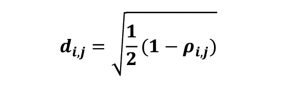
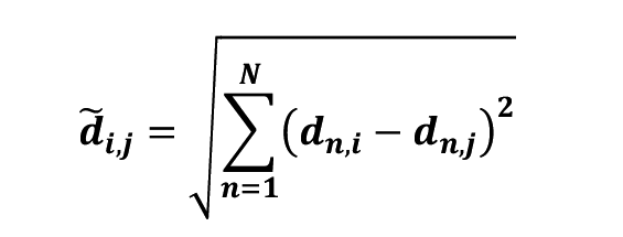
Since the above definition uses only the relationship between the two companies, to incorporate the correlation between the two or more companies as well, the following distance are used as the clustering distance. This method is the approach used in Prado's HRP method[2], [3], [4]. HRP method is widely used in portfolio development. Finally, the distance between the two companies are calculated as follows where N is the total number of companies, 28 in this case.
3.2 Result by HRP
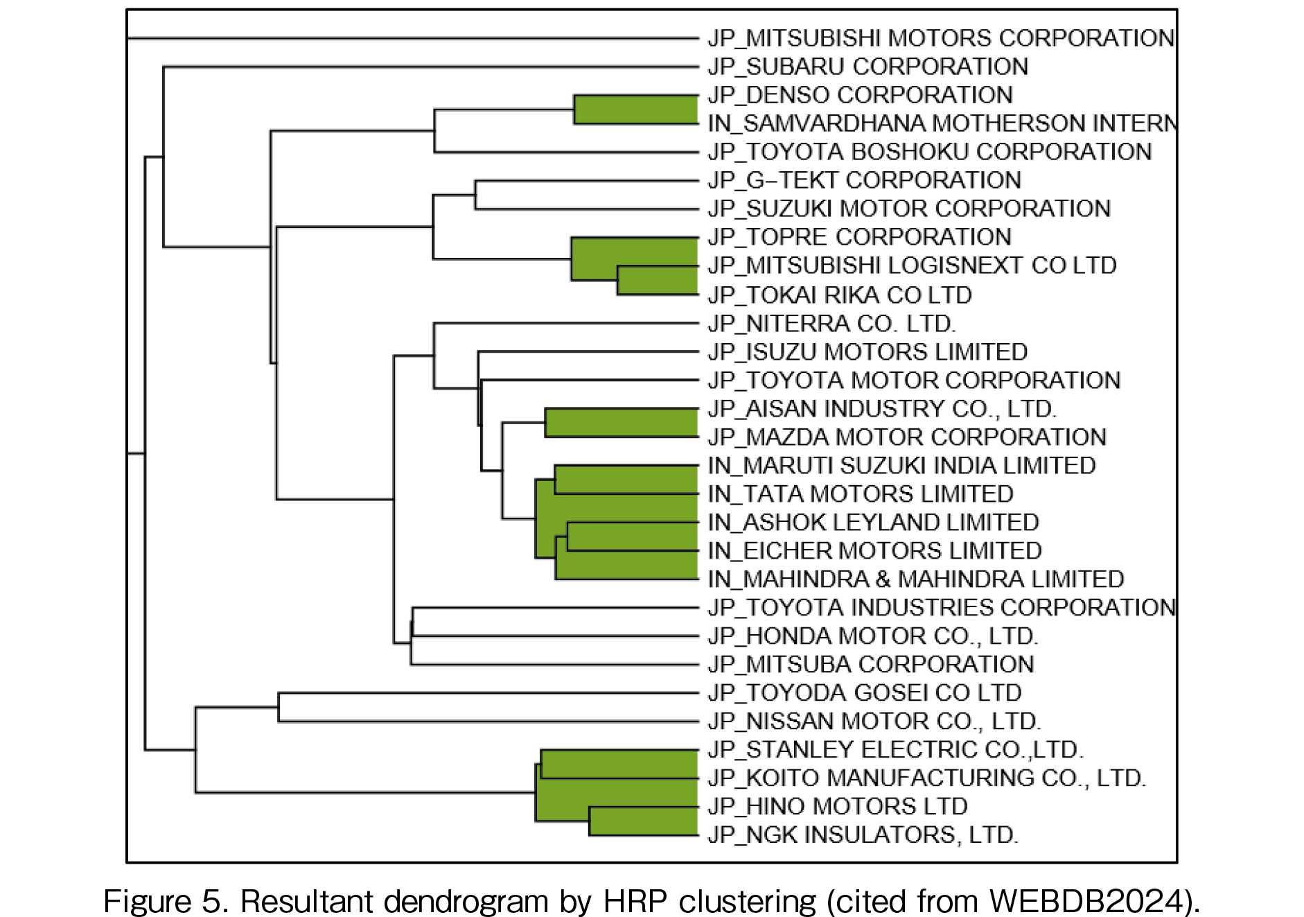
The feature of HRP distance is an adoption of the correlation coefficients. In the calculation of the correlation coefficients, standardization was conducted and the growth rate amplitude data are deleted. Only the correlation coefficient is used to evaluate the similarity. When we see the pattern similarity after the data standardization, the five Indian companies comprise a cluster: they are Maruti Suzuki, Tata, Ashok, Eicher, and Mahindra & Mahindra (see Figure 5). In the dendrogram in Figure 5, the clusters are colored at appropriate distance thresholds for proper visualization of the clusters. In the center of Figure 5, we find the cluster of Indian firms. Tracing the raw MC movement of the Indian automakers in Figure 1, Maruti Suzuki has been the leader among them since March 2020. Tata's MC has increased significantly since March 2023, and it is in second place behind Maruti Suzuki. The momentum of the increase suggests that Tata is becoming closer to Maruti Suzuki. SAMVARDHANA MOTHERSON INTERNATIONAL (Samvardhana) did not belong to this cluster (see Figure 5). The other five Indian companies’ movements show that the MC increased steadily throughout the period, although it declined once in March 2022. This is the trend for major Indian companies. On the other hand, Sambardhana peaked in June 2021 and continued to decline until March 2023, after which it continued to increase. This pattern is different from that of the other five companies. Sambardana is a component supplier that develops, manufactures, and sells components, systems, and modules for passenger cars/commercial vehicles in North America, South America, Europe, South Africa, the Middle East, Asia Pacific, Australia, and other regions. The five aforementioned companies differ in that they have India as their primary target market rather than global expansion. The difference in the market is considered to be reflected in the difference in the pattern of MC movements.
From this result and the raw MC data, it can be inferred that this cluster of five Indian firms is a cluster with high resilience. The hypothesis is that the cluster with high pattern similarity was formed because of the high stock price resilience, compared to the Japanese firms. For details, an analysis by Amplitude-based clustering has been done.
4. Amplitude-based Clustering Analysis
In this section, we shall explain the Amplitude-based clustering method. Then using the result of the clustering, dimensionality reduction is conducted, so that we can obtain the measurement of the recovery/resilience levels.
4.1 Amplitude-based Clustering Method
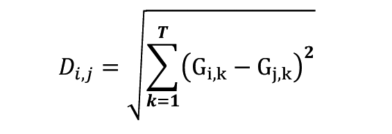
We now define and describe Amplitude-based clustering method. The details are described in [5], [6], [7]. For the distance definition of Amplitude-based clustering, we use Euclidean distance, given by
 【189頁】
where Gi,k is the index data of j-th company on k-th day and T is the number of sales days. Then the distance-distance between company I and j matrix is defined as follows:
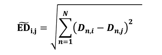
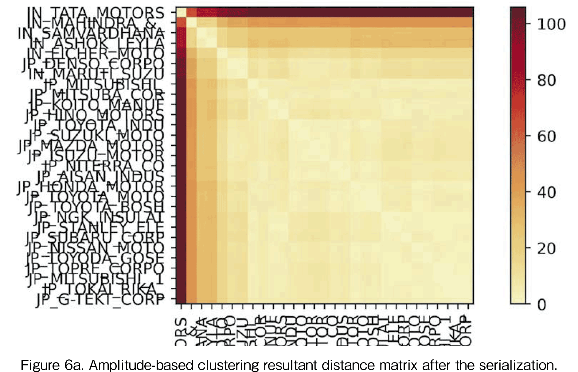
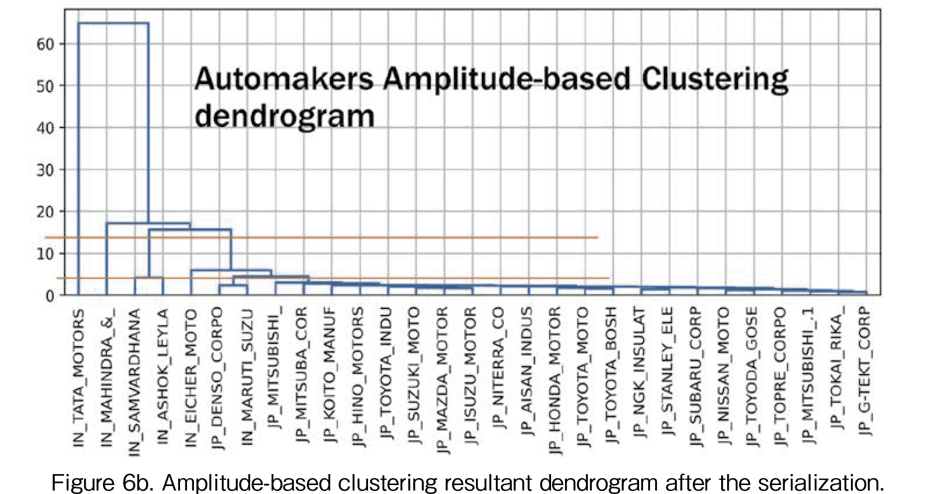
where N is the number of companies. Then we perform a hierarchical clustering based on the matrix  and we perform quasi-diagonalization on the distance-distance matrix. The resultant distance matrix is shown in Figure 6a. Its dendrogram is illustrated in Figure 6b. There the company list order is changed by the matrix serialization. The matrix serialization algorithm is described in [3]. In Figure 6a, the distance 0 is colored in white, and red means a large distance. Thus, the diagonal of the distance-distance matrix is zero. From the distance matrix in Figure 6a, it is found that Tata’s movement is extremely different from the others. In the dendrogram in Figure 6b, the vertical axis represents the distance between companies. This dendrogram also illustrates that Tata’s pattern is quite different from the others.
Next, we would like to find the recovery/growth measurement of the MC. For the measurement, we will conduct dimensionality reduction.
4.2 Dimensionality Reduction Method
In this section, we shall explain three-dimensionality reduction methods which are (1) Principal Component Analysis (PCA) [8] [9], (2) t-SNE [10] [11], and (3) UMAP [12] [13] [14] [15].
PCA (Principal Component Analysis) is a linear technique that works best with data that has a linear structure. It seeks to identify the underlying principal components in the data by projecting onto lower dimensions, minimizing variance, and preserving large pairwise distances. The variance-covariance matrix of the data is first calculated and the eigenvectors of the matrix correspond to each principal component of the data are found.
t-SNE is a nonlinear technique that focuses on preserving the pairwise similarities between data points in a lower-dimensional space [16]. In t-SNE, when calculating pairwise distances in the lower-dimensional space, t-distribution is used instead of the Gaussian (normal) distribution. The reason for this is that the t-distribution has heavier tails, which prevents distant points from being excessively pulled together. Compared to the Gaussian distribution, the t-distribution allows distant points to retain some level of similarity, leading to more natural clustering in the lower-dimensional space. t-SNE is a probabilistic method focused on preserving pairwise similarities between data points. It calculates the pairwise distances in the high-dimensional space and aims to faithfully reproduce these similarities when mapping them to a lower-dimensional space. t-SNE excels at preserving local structures (relationships between nearby data points), but it may not accurately represent the overall data structure (relationships between larger clusters).
On the other hand, UMAP is based on concepts from topology and Riemannian geometry, assuming that data lies on a low-dimensional manifold. UMAP captures the local topological structure of the data 【191頁】 in the high-dimensional space and maps it to a lower-dimensional space. This method often produces a more balanced representation of both the overall and local data structures compared to t-SNE.
4.3 Dimensionality Reduction Results
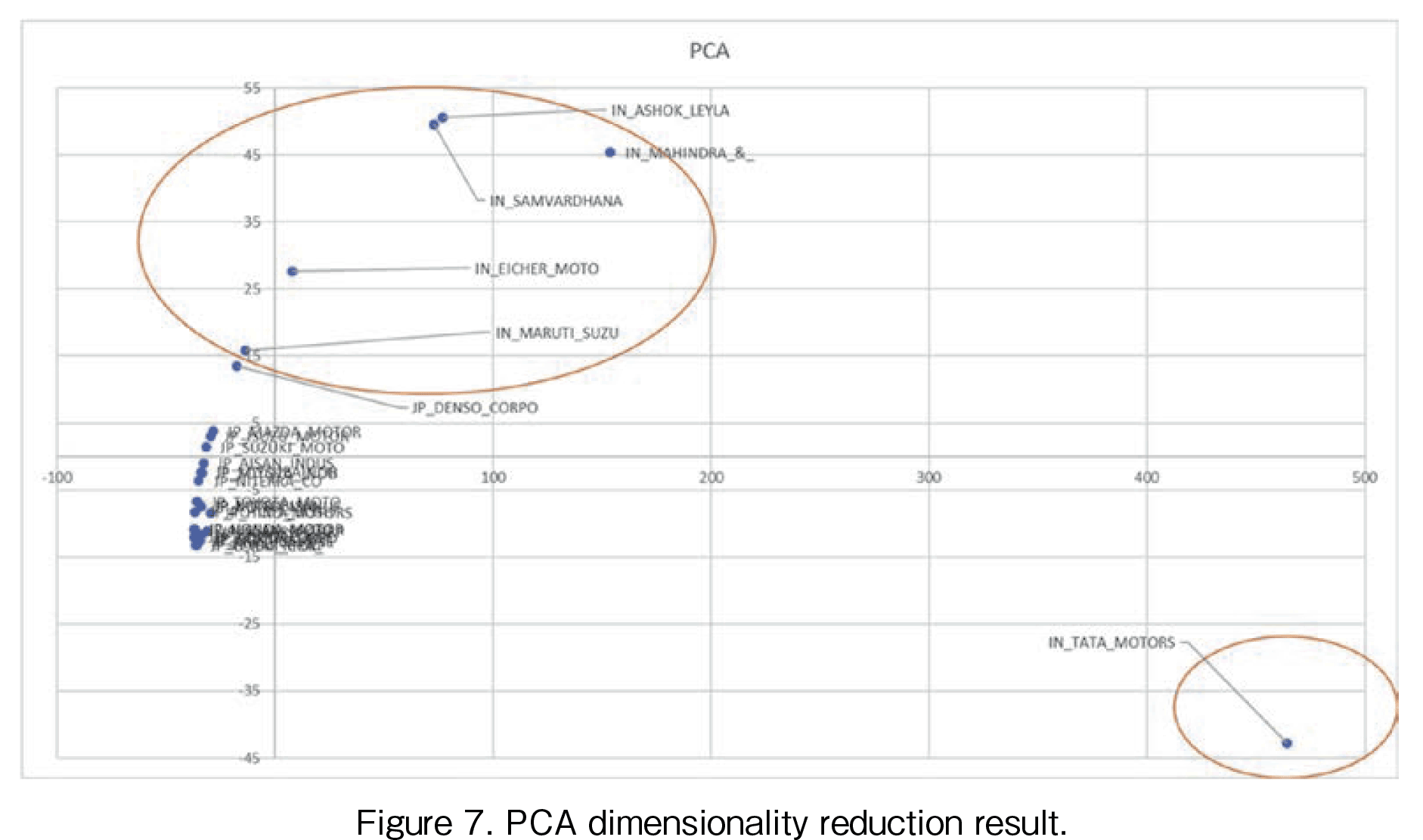
In this section, the comparison of the results by the three-dimensionality reduction methods, PCA, t-SNE, and UMAP are presented. Figure 7 illustrates the result by PCA. The first (horizontal) PCA axis can be thought of as the growth rate. The highest-growing companies from Figure 2 to 4 were (1) Tata, (2) Mahindra & Mahindra, (3) Ashok, (4) Samvardhana, (5) Eicher, and (6) Maruti Suzuki. As shown in Figure 7, the first PCA values are in the same order as that in Figures 2 to 4. We can say the first PCA values can express the growth levels. Among the Indian companies, especially the growth rate of Tata is extremely large. Although the first PCA axis can be clearly interpreted, it is difficult to interpret the meaning of the second (vertical) PCA axis. The reason why only the second value of Tata is negative remains unclear.
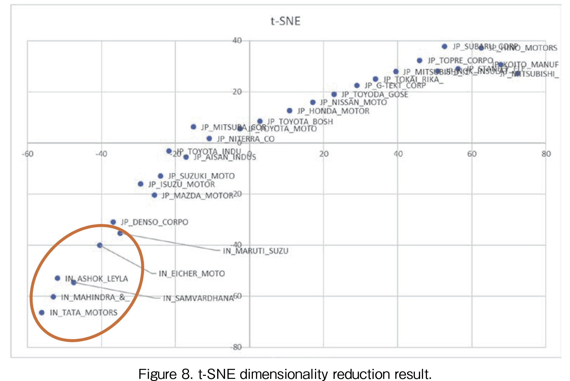
The result by t-SNE is shown in Figure 8. The lower first t-SNE value corresponds to the larger growth rate. Following the first t-SNE axis, the highest Indian companies are listed as (1) Tata, (2) Mahindra & Mahindra, (3) Ashok, (4) Samvardhana, (5) Eicher, and (6) Maruti Suzuki. However, before Murti Suzuki, there was Denso, which may be derived from Denso’s peak in December 2021. The ranking order by the first t-SNE is almost the same as the ranking order by the second t-SNE. The difference may be the first t-SNE value means the average ranking and that the second t-SNE value does recovery/growth rate.
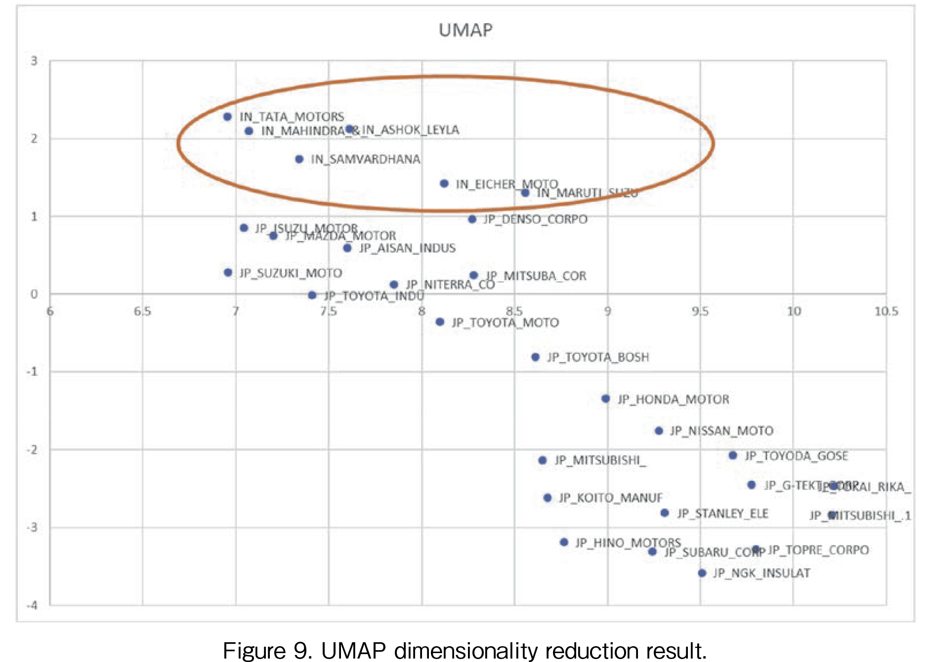
The third dimensional deduction method is UMAP. In Figure 9, the result by UMAP is shown. It is unclear how the first (horizontal) UMAP axis should be evaluated. However, the second (vertical) UMAP axis can be interpreted as the growth rate: the larger the second UMAP value, the higher the growth rate, the order is the same as (1) Tata, (2) Mahindra & Mahindra, (3) Ashok, (4) Samvardhana, (5) Eicher, and (6) Maruti Suzuki.
In this section, the discussion concerning the result of comparison is conducted.
Our objective was to extract a measurement of growth rates from the dimensionality reduction techniques. As a result, all three kinds of dimensionality reduction methods can offer the axis which can express the growth rate. They are (1) the first PCA axis, (2) the second t-SNE axis, and (3) the second UMAP axis. In this result, it is hard to interpret the second PCA axis and the first UMAP axis. The difficulties are derived from the complexity of the mapping to the two-dimensional world. The source data of the distance are Euclid distance of the indexed data. The distance value includes the time series variance changes. Therefore, it is not easy to evaluate the two company patterns' similarity just from the distance value. Therefore, we cannot clearly interpret the meaning of the first UMAP axis.
As a result, we can say that the Indian automaker's recovery/growth rates after COVID-19 were much higher than those of Japanese automakers. All three methods' results showed the larger MC growth of the Indian automakers, compared to that of Japanese automakers.
We use hierarchical clustering to analyze the pattern of market capitalization fluctuations in the Indian auto manufacturing industry. However, the Indian automotive manufacturing industry showed a quick stock price resilience, and performed better than in the pre-COVID-19 period. In the clustering process, we compared the Indian and Japanese automobile manufacturing industries, and found that the five leading Indian firms are extracted as a cluster with the similar pattern. This indicates that the Indian firms have a remarkable pattern of fluctuation that differs from that of the Japanese firms. This is thought to be due to the increase in purchasing power resulting from the increase in the middle-income class accompanying the increase in India's GDP, as well as the effects of the Indian government's policy to promote the manufacturing industry. We will continue our analysis, including the growth of the growth rate.
Acknowledgments
This research was partly supported by a special project of Gakushuin University Computer Centre in 2024.
【194頁】[1] B. Chakraborty, Y. Shirota, and B. Sreekanth, "India Automakers Market Capital Movement Pattern Clustering," Research Report of Information Processing Society of Japan, IPSJ SIG Technical Report, vol. in printing, 2024.
[2] D. P. M. Lopez, "Building diversified portfolios that outperform out of sample," The Journal of Portfolio Management, vol. 42, no. 4, pp. 59-69, 2016.
[3] M. L. De Prado, Advances in financial machine learning John Wiley & Sons, 2018.
[4] M. M. L. de Prado, Machine learning for asset managers Cambridge University Press, 2020.
[5] Y. Shirota and B. Chakraborty, "Amplitude-Based Time Series Data Clustering Method," Gakushuin Economics Papers, vol. 59, no. 2, pp. 127-140, 2022.
[6] 高畠早紀 and 白田由香利,"利上げによる米国企業時価総額への影響分析 〜 Amplitude-based clusteringによる時系列分析 〜," 電子情報通信学会技術研究報告,pp. 1-5, 2023.
[7] S. Matsuhashi and Y. Shirota, "Resilience Evaluation of Automakers After 2008 Financial Crisis by UMAP," International Journal of Machine Learning, vol. 13, no. 3, pp. 125-130 2023.
[8] C. M. Bishop and N. M. Nasrabadi, Pattern recognition and machine learning Springer, 2006.
[9] T. Hastie, R. Tibshirani, J. H. Friedman, and J. H. Friedman, The elements of statistical learning: data mining, inference, and prediction Springer, 2009.
[10] L. Van der Maaten and G. Hinton, "Visualizing data using t-SNE," Journal of machine learning research, vol. 9, no. 11, 2008.
[11] L. Van Der Maaten, "Accelerating t-SNE using tree-based algorithms," The Journal of Machine Learning Research, vol. 15, no. 1, pp. 3221-3245, 2014.
[12] L. McInnes, "UMAP: Uniform Manifold Approximation and Projection for Dimension Reduction — umap 0.5 documentation," 2018. [Online]
[13] A. Coenen and A. Pearce, "Understanding UMAP; 2019," URL https://pair-code. github. io/understanding-umap.
[14] A. Coenen and A. Pearce, "Understanding umap," Google PAIR, 2019.
[15] L. McInnes, "UMAP: Uniform Manifold Approximation and Projection for Dimension Reduction." [Online]. Available: https://umap-learn.readthedocs.io/en/latest/
[16] A. A. Awan, "Introduction to t-SNE," 2023. [Online]. Available: https://www.datacamp.com/tutorial/introduction-t-sne